
Hidden Markov Model - Implemented from scratch
Introduction
The Internet is full of good articles that explain the theory behind the Hidden Markov Model (HMM) well (e.g. 1, 2, 3 and 4) . However, many of these works contain a fair amount of rather advanced mathematical equations. While equations are necessary if one wants to explain the theory, we decided to take it to the next level and create a gentle step by step practical implementation to complement the good work of others.
In this short series of two articles, we will focus on translating all of the complicated mathematics into code. Our starting point is the document written by Mark Stamp. We will use this paper to define our code (this article) and then use a somewhat peculiar example of “Morning Insanity” to demonstrate its performance in practice.
Notation
Before we begin, let’s revisit the notation we will be using. By the way, don’t worry if some of that is unclear to you. We will hold your hand.
- - length of the observation sequence.
- - number of latent (hidden) states.
- - number of observables.
- - hidden states.
- - set of possible observations.
- - state transition matrix.
- - emission probability matrix.
- - initial state probability distribution.
- - observation sequence.
- - hidden state sequence.
Having that set defined, we can calculate the probability of any state and observation using the matrices:
- - begin an transition matrix.
- - being an emission matrix.
The probabilities associated with transition and observation (emission) are:
- ,
- .
The model is therefore defined as a collection: .
Fundamental definitions
Since HMM is based on probability vectors and matrices, let’s first define objects that will represent the fundamental concepts. To be useful, the objects must reflect on certain properties. For example, all elements of a probability vector must be numbers and they must sum up to 1. Therefore, let’s design the objects the way they will inherently safeguard the mathematical properties.
1
2
3
4
5
6
7
8
9
10
11
12
13
14
15
16
17
18
19
20
21
22
23
24
25
26
27
28
29
30
31
32
33
34
35
36
37
38
39
40
41
42
43
44
45
46
47
48
49
50
51
52
53
54
55
56
57
58
59
60
61
62
63
64
65
66
67
68
69
70
71
72
73
74
75
76
77
78
79
80
81
import numpy as np
import pandas as pd


class ProbabilityVector:
    def __init__(self, probabilities: dict):
        states = probabilities.keys()
        probs  = probabilities.values()

        assert len(states) == len(probs),
            "The probabilities must match the states."
        assert len(states) == len(set(states)),
            "The states must be unique."
        assert abs(sum(probs) - 1.0) < 1e-12,
            "Probabilities must sum up to 1."
        assert len(list(filter(lambda x: 0 <= x <= 1, probs))) == len(probs), \
            "Probabilities must be numbers from [0, 1] interval."

        self.states = sorted(probabilities)
        self.values = np.array(list(map(lambda x:
            probabilities[x], self.states))).reshape(1, -1)

    @classmethod
    def initialize(cls, states: list):
        size = len(states)
        rand = np.random.rand(size) / (size**2) + 1 / size
        rand /= rand.sum(axis=0)
        return cls(dict(zip(states, rand)))

    @classmethod
    def from_numpy(cls, array: np.ndarray, state: list):
        return cls(dict(zip(states, list(array))))

    @property
    def dict(self):
        return {k:v for k, v in zip(self.states, list(self.values.flatten()))}

    @property
    def df(self):
        return pd.DataFrame(self.values, columns=self.states, index=['probability'])

    def __repr__(self):
        return "P({}) = {}.".format(self.states, self.values)

    def __eq__(self, other):
        if not isinstance(other, ProbabilityVector):
            raise NotImplementedError
        if (self.states == other.states) and (self.values == other.values).all():
            return True
        return False

    def __getitem__(self, state: str) -> float:
        if state not in self.states:
            raise ValueError("Requesting unknown probability state from vector.")
        index = self.states.index(state)
        return float(self.values[0, index])

    def __mul__(self, other) -> np.ndarray:
        if isinstance(other, ProbabilityVector):
            return self.values * other.values
        elif isinstance(other, (int, float)):
            return self.values * other
        else:
            NotImplementedError

    def __rmul__(self, other) -> np.ndarray:
        return self.__mul__(other)

    def __matmul__(self, other) -> np.ndarray:
        if isinstance(other, ProbabilityMatrix):
            return self.values @ other.values

    def __truediv__(self, number) -> np.ndarray:
        if not isinstance(number, (int, float)):
            raise NotImplementedError
        x = self.values
        return x / number if number != 0 else x / (number + 1e-12)

    def argmax(self):
        index = self.values.argmax()
        return self.states[index]
The most natural way to initialize this object is to use a dictionary as it associates values with unique keys. Dictionaries, unfortunately, do not provide any assertion mechanisms that put any constraints on the values. Consequently, we build our custom ProbabilityVector object to ensure that our values behave correctly. Most importantly, we enforce the following:
- The number of values must equal the number of the keys (names of our states). Although this is not a problem when initializing the object from a dictionary, we will use other ways later.
- All names of the states must be unique (the same arguments apply).
- The probabilities must sum up to 1 (up to a certain tolerance).
- All probabilities must be .
Having ensured that, we also provide two alternative ways to instantiate ProbabilityVector objects (decorated with @classmethod).
- We instantiate the objects randomly - it will be useful when training.
- We use ready-made numpy arrays and use values therein, and only providing the names for the states.
For convenience and debugging, we provide two additional methods for requesting the values.
Decorated with @property, they return the content of the PV object as a dictionary or a pandas dataframe.
The PV objects need to satisfy the following mathematical operations (for the purpose of constructing of HMM):
- comparison (
__eq__) - to know if any two PV’s are equal, - element-wise multiplication of two PV’s or multiplication with a scalar (
__mul__and__rmul__). - dot product (
__matmul__) - to perform vector-matrix multiplication - division by number (
__truediv__), argmaxto find for which state the probability is the highest.__getitem__to enable selecting value by the key.
Note that when e.g. multiplying a PV with a scalar, the returned structure is a resulting numpy array, not another PV. This is because multiplying by anything other than 1 would violate the integrity of the PV itself.
Internally, the values are stored as a numpy array of size .
Example
1
2
3
4
5
6
7
8
9
10
11
12
13
14
15
16
17
18
19
20
a1 = ProbabilityVector({'rain': 0.7, 'sun': 0.3})
a2 = ProbabilityVector({'sun': 0.1, 'rain': 0.9})
print(a1.df)
print(a2.df)

print("Comparison:", a1 == a2)
print("Element-wise multiplication:", a1 * a2)
print("Argmax:", a1.argmax())
print("Getitem:", a1['rain'])

# OUTPUT
>>>              rain  sun
    probability   0.7  0.3
>>>              rain  sun
    probability   0.9  0.1

>>> Comparison: False
>>> Element-wise multiplication: [[0.63 0.03]]
>>> Argmax: rain
>>> Getitem: 0.7
Probability Matrix
Another object is a Probability Matrix, which is a core part of the HMM definition.
Formally, the and matrices must be row-stochastic, meaning that the values of every row must sum up to 1.
We can, therefore, define our PM by stacking several PV’s, which we have constructed in a way to guarantee this constraint.
1
2
3
4
5
6
7
8
9
10
11
12
13
14
15
16
17
18
19
20
21
22
23
24
25
26
27
28
29
30
31
32
33
34
35
36
37
38
39
40
41
42
43
44
45
class ProbabilityMatrix:
    def __init__(self, prob_vec_dict: dict):

        assert len(prob_vec_dict) > 1, \
            "The numebr of input probability vector must be greater than one."
        assert len(set([str(x.states) for x in prob_vec_dict.values()])) == 1, \
            "All internal states of all the vectors must be indentical."
        assert len(prob_vec_dict.keys()) == len(set(prob_vec_dict.keys())), \
            "All observables must be unique."

        self.states      = sorted(prob_vec_dict)
        self.observables = prob_vec_dict[self.states[0]].states
        self.values      = np.stack([prob_vec_dict[x].values for x in self.states]).squeeze()

    @classmethod
    def initialize(cls, states: list, observables: list):
        size = len(states)
        rand = np.random.rand(size, len(observables)) / (size**2) + 1 / size
        rand /= rand.sum(axis=1).reshape(-1, 1)
        aggr = [dict(zip(observables, rand[i, :])) for i in range(len(states))]
        pvec = [ProbabilityVector(x) for x in aggr]
        return cls(dict(zip(states, pvec)))

    @classmethod
    def from_numpy(cls, array: np.ndarray, states: list, observables: list):
        p_vecs = [ProbabilityVector(dict(zip(observables, x))) for x in array]
        return cls(dict(zip(states, p_vecs)))

    @property
    def dict(self):
        return self.df.to_dict()

    @property
    def df(self):
        return pd.DataFrame(self.values, columns=self.observables, index=self.states)

    def __repr__(self):
        return "PM {} states: {} -> obs: {}.".format(
            self.values.shape, self.states, self.observables)

    def __getitem__(self, observable: str) -> np.ndarray:
        if observable not in self.observables:
            raise ValueError("Requesting unknown probability observable from the matrix.")
        index = self.observables.index(observable)
        return self.values[:, index].reshape(-1, 1)
Here, the way we instantiate PM’s is by supplying a dictionary of PV’s to the constructor of the class. By doing this, we not only ensure that every row of PM is stochastic, but also supply the names for every observable.
| Our PM can, therefore, give an array of coefficients for any observable. |
Mathematically, the PM is a matrix:
The other methods are implemented in similar way to PV.
Example
1
2
3
4
5
6
7
8
9
10
11
12
13
14
15
16
17
18
19
20
21
22
23
24
25
26
27
28
29
30
31
32
33
34
a1 = ProbabilityVector({'rain': 0.7, 'sun': 0.3})
a2 = ProbabilityVector({'rain': 0.6, 'sun': 0.4})
A  = ProbabilityMatrix({'hot': a1, 'cold': a2})

print(A)
print(A.df)
>>> PM (2, 2) states: ['cold', 'hot'] -> obs: ['rain', 'sun'].
>>>      rain  sun
   cold   0.6  0.4
   hot    0.7  0.3

b1 = ProbabilityVector({'0S': 0.1, '1M': 0.4, '2L': 0.5})
b2 = ProbabilityVector({'0S': 0.7, '1M': 0.2, '2L': 0.1})
B =  ProbabilityMatrix({'0H': b1, '1C': b2})

print(B)
print(B.df)
>>> PM (2, 3) states: ['0H', '1C'] -> obs: ['0S', '1M', '2L'].
>>>       0S   1M   2L
     0H  0.1  0.4  0.5
     1C  0.7  0.2  0.1

P = ProbabilityMatrix.initialize(list('abcd'), list('xyz'))
print('Dot product:', a1 @ A)
print('Initialization:', P)
print(P.df)
>>> Dot product: [[0.63 0.37]]
>>> Initialization: PM (4, 3)
    states: ['a', 'b', 'c', 'd'] -> obs: ['x', 'y', 'z'].
>>>          x         y         z
   a  0.323803  0.327106  0.349091
   b  0.318166  0.326356  0.355478
   c  0.311833  0.347983  0.340185
   d  0.337223  0.316850  0.345927
Implementing Hidden Markov Chain
Before we proceed with calculating the score, let’s use our PV and PM definitions to implement the Hidden Markov Chain.
Again, we will do so as a class, calling it HiddenMarkovChain. It will collate at , and .
Later on, we will implement more methods that are applicable to this class.
Computing score
Computing the score means to find what is the probability of a particular chain of observations given our (known) model . In other words, we are interested in finding .
We can find by marginalizing all possible chains of the hidden variables , where :
Since (the product of all probabilities related to the observables) and (the product of all probabilities of transitioning from to , the probability we are looking for (the score) is:
This is a naive way of computing of the score, since we need to calculate the probability for every possible chain . Either way, let’s implement it in python:
1
2
3
4
5
6
7
8
9
10
11
12
13
14
15
16
17
18
19
20
21
22
23
24
25
26
27
28
29
30
31
32
33
34
35
36
37
38
39
40
41
from itertools import product
from functools import reduce


class HiddenMarkovChain:
    def __init__(self, T, E, pi):
        self.T = T  # transmission matrix A
        self.E = E  # emission matrix B
        self.pi = pi
        self.states = pi.states
        self.observables = E.observables

    def __repr__(self):
        return "HML states: {} -> observables: {}.".format(
            len(self.states), len(self.observables))

    @classmethod
    def initialize(cls, states: list, observables: list):
        T = ProbabilityMatrix.initialize(states, states)
        E = ProbabilityMatrix.initialize(states, observables)
        pi = ProbabilityVector.initialize(states)
        return cls(T, E, pi)

    def _create_all_chains(self, chain_length):
        return list(product(*(self.states,) * chain_length))

    def score(self, observations: list) -> float:
        def mul(x, y): return x * y

        score = 0
        all_chains = self._create_all_chains(len(observations))
        for idx, chain in enumerate(all_chains):
            expanded_chain = list(zip(chain, [self.T.states[0]] + list(chain)))
            expanded_obser = list(zip(observations, chain))

            p_observations = list(map(lambda x: self.E.df.loc[x[1], x[0]], expanded_obser))
            p_hidden_state = list(map(lambda x: self.T.df.loc[x[1], x[0]], expanded_chain))
            p_hidden_state[0] = self.pi[chain[0]]

            score += reduce(mul, p_observations) * reduce(mul, p_hidden_state)
        return score
Example
1
2
3
4
5
6
7
8
9
10
11
12
13
14
15
a1 = ProbabilityVector({'1H': 0.7, '2C': 0.3})
a2 = ProbabilityVector({'1H': 0.4, '2C': 0.6})

b1 = ProbabilityVector({'1S': 0.1, '2M': 0.4, '3L': 0.5})
b2 = ProbabilityVector({'1S': 0.7, '2M': 0.2, '3L': 0.1})

A = ProbabilityMatrix({'1H': a1, '2C': a2})
B = ProbabilityMatrix({'1H': b1, '2C': b2})
pi = ProbabilityVector({'1H': 0.6, '2C': 0.4})

hmc = HiddenMarkovChain(A, B, pi)
observations = ['1S', '2M', '3L', '2M', '1S']

print("Score for {} is {:f}.".format(observations, hmc.score(observations)))
>>> Score for ['1S', '2M', '3L', '2M', '1S'] is 0.003482.
If our implementation is correct, then all score values for all possible observation chains, for a given model should add up to one. Namely:
1
2
3
4
5
6
all_possible_observations = {'1S', '2M', '3L'}
chain_length = 3  # any int > 0
all_observation_chains = list(product(*(all_possible_observations,) * chain_length))
all_possible_scores = list(map(lambda obs: hmc.score(obs), all_observation_chains))
print("All possible scores added: {}.".format(sum(all_possible_scores)))
>>> All possible scores added: 1.0.
Indeed.
Score with forward-pass
Computing the score the way we did above is kind of naive. In order to find the number for a particular observation chain , we have to compute the score for all possble latent variable sequences . That requries multiplications, which even for small numbers takes time.
Another way to do it is to calculate partial observations of a sequence up to time .
For and :
Consequently,
and
Then
Note that is a vector of lenght . The sum of the product can, in fact, be written as a dot product. Therefore:
where by we denote an element-wise multiplication.
With this implementation, we reduce the number of multiplication to and can take advantage of vectorization.
1
2
3
4
5
6
7
8
9
10
11
12
class HiddenMarkovChain_FP(HiddenMarkovChain):
    def _alphas(self, observations: list) -> np.ndarray:
        alphas = np.zeros((len(observations), len(self.states)))
        alphas[0, :] = self.pi.values * self.E[observations[0]].T
        for t in range(1, len(observations)):
            alphas[t, :] = (alphas[t - 1, :].reshape(1, -1)
                         @ self.T.values) * self.E[observations[t]].T
        return alphas

    def score(self, observations: list) -> float:
        alphas = self._alphas(observations)
        return float(alphas[-1].sum())
Example
1
2
3
4
5
hmc_fp = HiddenMarkovChain_FP(A, B, pi)

observations = ['1S', '2M', '3L', '2M', '1S']
print("Score for {} is {:f}.".format(observations, hmc_fp.score(observations)))
>>> All possible scores added: 1.0.
…yup.
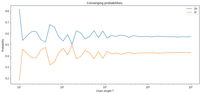
Simulation and convergence
Let’s test one more thing. Basically, let’s take our and use it to generate a sequence of random observables, starting from some initial state probability .
If the desired length is “large enough”, we would expect that the system to converge on a sequence that, on average, gives the same number of events as we would expect from and matrices directly. In other words, the transition and the emission matrices “decide”, with a certain probability, what the next state will be and what observation we will get, for every step, respectively. Therefore, what may initially look like random events, on average should reflect the coefficients of the matrices themselves. Let’s check that as well.
1
2
3
4
5
6
7
8
9
10
11
12
13
14
15
16
17
18
class HiddenMarkovChain_Simulation(HiddenMarkovChain):
    def run(self, length: int) -> (list, list):
        assert length >= 0, "The chain needs to be a non-negative number."
        s_history = [0] * (length + 1)
        o_history = [0] * (length + 1)

        prb = self.pi.values
        obs = prb @ self.E.values
        s_history[0] = np.random.choice(self.states, p=prb.flatten())
        o_history[0] = np.random.choice(self.observables, p=obs.flatten())

        for t in range(1, length + 1):
            prb = prb @ self.T.values
            obs = prb @ self.E.values
            s_history[t] = np.random.choice(self.states, p=prb.flatten())
            o_history[t] = np.random.choice(self.observables, p=obs.flatten())

        return o_history, s_history
Example
1
2
3
4
5
hmc_s = HiddenMarkovChain_Simulation(A, B, pi)
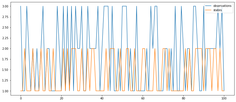
observation_hist, states_hist = hmc_s.run(100) # length = 1000
stats = pd.DataFrame({
'observations': observation_hist,
'states': states_hist}).applymap(lambda x: int(x[0])).plot()
Latent states
The state matrix is given by the following coefficients:
Consequently, the probability of “being” in the state at , regardless of the previous state, is equal to:
If we assume that the prior probabilities of being at some state at are totally random, then and , which after renormalizing give 0.55 and 0.45, respectively.
If we cound the number of occurences of each state and divide it by the number of elements in our sequence, we would get closer and closer to these number as the lenght of the sequence grows.
Example
1
2
3
4
5
6
7
8
9
10
11
12
13
14
15
16
17
18
hmc_s = HiddenMarkovChain_Simulation(A, B, pi)

stats = {}
for length in np.logspace(1, 5, 40).astype(int):
    observation_hist, states_hist = hmc_s.run(length)
    stats[length] = pd.DataFrame({
        'observations': observation_hist,
        'states': states_hist}).applymap(lambda x: int(x[0]))

S = np.array(list(map(lambda x:
        x['states'].value_counts().to_numpy() / len(x), stats.values())))

plt.semilogx(np.logspace(1, 5, 40).astype(int), S)
plt.xlabel('Chain length T')
plt.ylabel('Probability')
plt.title('Converging probabilities.')
plt.legend(['1H', '2C'])
plt.show()
Uncovering hidden variables
Let’s take our HiddenMarkovChain class to the next level and supplement it with more methods.
The methods will help us to discover the most probable sequence of hidden variables behind the observation sequence.
Expanding the class
We have defined to be the probability of partial observation of the sequence up to time .
Now, let’s define the “opposite” probability. Namely, the probability of observing the sequence from down to .
For and , we define:
As before, we can calulate recursively:
Then for :
which in vectorized form, will be:
Finally, we also define a new quantity to indicate the state at time , for which the probability (calculated forwards and backwards) is the maximum:
Consequently, for any step , the state of the maximum likelihood can be found using:
1
2
3
4
5
6
7
8
9
10
11
12
13
14
15
16
17
18
19
20
21
22
class HiddenMarkovChain_Uncover(HiddenMarkovChain_Simulation):
    def _alphas(self, observations: list) -> np.ndarray:
        alphas = np.zeros((len(observations), len(self.states)))
        alphas[0, :] = self.pi.values * self.E[observations[0]].T
        for t in range(1, len(observations)):
            alphas[t, :] = (alphas[t - 1, :].reshape(1, -1) @ self.T.values) \
                         * self.E[observations[t]].T
        return alphas

    def _betas(self, observations: list) -> np.ndarray:
        betas = np.zeros((len(observations), len(self.states)))
        betas[-1, :] = 1
        for t in range(len(observations) - 2, -1, -1):
            betas[t, :] = (self.T.values @ (self.E[observations[t + 1]] \
                        * betas[t + 1, :].reshape(-1, 1))).reshape(1, -1)
        return betas

    def uncover(self, observations: list) -> list:
        alphas = self._alphas(observations)
        betas = self._betas(observations)
        maxargs = (alphas * betas).argmax(axis=1)
        return list(map(lambda x: self.states[x], maxargs))
Validation
To validate, let’s generate some observable sequence .
For that, we can use our model’s .run method.
Then, we will use the .uncover method to find the most likely latent variable sequence.
Example
1
2
3
4
5
6
7
8
9
10
11
12
13
14
np.random.seed(42)

a1 = ProbabilityVector({'1H': 0.7, '2C': 0.3})
a2 = ProbabilityVector({'1H': 0.4, '2C': 0.6})
b1 = ProbabilityVector({'1S': 0.1, '2M': 0.4, '3L': 0.5})
b2 = ProbabilityVector({'1S': 0.7, '2M': 0.2, '3L': 0.1})
A  = ProbabilityMatrix({'1H': a1, '2C': a2})
B  = ProbabilityMatrix({'1H': b1, '2C': b2})
pi = ProbabilityVector({'1H': 0.6, '2C': 0.4})

hmc = HiddenMarkovChain_Uncover(A, B, pi)

observed_sequence, latent_sequence = hmc.run(5)
uncovered_sequence = hmc.uncover(observed_sequence)
| 0 | 1 | 2 | 3 | 4 | 5 | |
|---|---|---|---|---|---|---|
| observed sequence | 3L | 3M | 1S | 3L | 3L | 3L |
| latent sequence | 1H | 2C | 1H | 1H | 2C | 1H |
| uncovered sequence | 1H | 1H | 2C | 1H | 1H | 1H |
As we can see, the most likely latent state chain (according to the algorithm) is not the same as the one that actually caused the observations. This is to be expected. Afterall, each observation sequence can only be manifested with certain probability, dependent on the latent sequence.
The code below, evaluates the likelihood of different latent sequences resulting in our observation sequence.
1
2
3
4
5
6
7
8
9
10
11
12
13
14
15
all_possible_states = {'1H', '2C'}
chain_length = 6  # any int > 0
all_states_chains = list(product(*(all_possible_states,) * chain_length))

df = pd.DataFrame(all_states_chains)
dfp = pd.DataFrame()

for i in range(chain_length):
    dfp['p' + str(i)] = df.apply(lambda x:
        hmc.E.df.loc[x[i], observed_sequence[i]], axis=1)

scores = dfp.sum(axis=1).sort_values(ascending=False)
df = df.iloc[scores.index]
df['score'] = scores
df.head(10).reset_index()
| index | 0 | 1 | 2 | 3 | 4 | 5 | score |
|---|---|---|---|---|---|---|---|
| 8 | 1H | 1H | 2C | 1H | 1H | 1H | 3.1 |
| 24 | 1H | 2C | 2C | 1H | 1H | 1H | 2.9 |
| 40 | 2C | 1H | 2C | 1H | 1H | 1H | 2.7 |
| 12 | 1H | 1H | 2C | 2C | 1H | 1H | 2.7 |
| 10 | 1H | 1H | 2C | 1H | 2C | 1H | 2.7 |
| 9 | 1H | 1H | 2C | 1H | 1H | 2C | 2.7 |
| 25 | 1H | 2C | 2C | 1H | 1H | 2C | 2.5 |
| 0 | 1H | 1H | 1H | 1H | 1H | 1H | 2.5 |
| 26 | 1H | 2C | 2C | 1H | 2C | 1H | 2.5 |
| 28 | 1H | 2C | 2C | 2C | 1H | 1H | 2.5 |
The result above shows the sorted table of the latent sequences, given the observation sequence. The actual latent sequence (the one that caused the observations) places itself on the 35th position (we counted index from zero).
1
2
3
4
5
dfc = df.copy().reset_index()
for i in range(chain_length):
    dfc = dfc[dfc[i] == latent_sequence[i]]

dfc
| index | 0 | 1 | 2 | 3 | 4 | 5 | score |
|---|---|---|---|---|---|---|---|
| 18 | 1H | 2C | 1H | 1H | 2C | 1H | 1.9 |
Training the model
The time has come to show the training procedure. Formally, we are interested in finding such that given a desired observation sequence , our model would give the best fit.
Expanding the class
Here, our starting point will be the HiddenMarkovModel_Uncover that we have defined earlier.
We will add new methods to train it.
Knowing our latent states and possible observation states , we automatically know the sizes of the matrices and , hence and . However, we need to determine and .
For and , we define “di-gammas”:
is the probability of transitioning . Writing it in terms of , we have:
Now, thinking in terms of implementation, we want to avoid looping over and at the same time, as it’s gonna be deadly slow. Fortunately, for every , we can vectorize the equation (preserving that are indexed with i while are indexed with ).
Having the equation for , we can calulate
To find , we do
- For :
or
- For :
- For and :
1
2
3
4
5
6
7
8
9
10
11
12
13
class HiddenMarkovLayer(HiddenMarkovChain_Uncover):
    def _digammas(self, observations: list) -> np.ndarray:
        L, N = len(observations), len(self.states)
        digammas = np.zeros((L - 1, N, N))

        alphas = self._alphas(observations)
        betas = self._betas(observations)
        score = self.score(observations)
        for t in range(L - 1):
            P1 = (alphas[t, :].reshape(-1, 1) * self.T.values)
            P2 = self.E[observations[t + 1]].T * betas[t + 1].reshape(1, -1)
            digammas[t, :, :] = P1 * P2 / score
        return digammas
Having the “layer” supplemented with the ._difammas method, we should be able to perform all the necessary calculations.
However, it makes sense to delegate the “management” of the layer to another class.
In fact, the model training can be summarized as follows:
- Initialize and .
- Calculate .
- Update the model’s and .
- We repeat the 2. and 3. until the score no longer increases.
1
2
3
4
5
6
7
8
9
10
11
12
13
14
15
16
17
18
19
20
21
22
23
24
25
26
27
28
29
30
31
32
33
34
35
36
37
38
39
40
41
42
43
44
45
46
47
class HiddenMarkovModel:
def __init__(self, hml: HiddenMarkovLayer):
self.layer = hml
self._score_init = 0
self.score_history = []
@classmethod
def initialize(cls, states: list, observables: list):
layer = HiddenMarkovLayer.initialize(states, observables)
return cls(layer)
def update(self, observations: list) -> float:
alpha = self.layer._alphas(observations)
beta = self.layer._betas(observations)
digamma = self.layer._digammas(observations)
score = alpha[-1].sum()
gamma = alpha * beta / score
L = len(alpha)
obs_idx = [self.layer.observables.index(x) for x in observations]
capture = np.zeros((L, len(self.layer.states), len(self.layer.observables)))
for t in range(L):
capture[t, :, obs_idx[t]] = 1.0
pi = gamma[0]
T = digamma.sum(axis=0) / gamma[:-1].sum(axis=0).reshape(-1, 1)
E = (capture * gamma[:, :, np.newaxis]).sum(axis=0) / gamma.sum(axis=0).reshape(-1, 1)
self.layer.pi = ProbabilityVector.from_numpy(pi, self.layer.states)
self.layer.T = ProbabilityMatrix.from_numpy(T, self.layer.states, self.layer.states)
self.layer.E = ProbabilityMatrix.from_numpy(E, self.layer.states, self.layer.observables)
return score
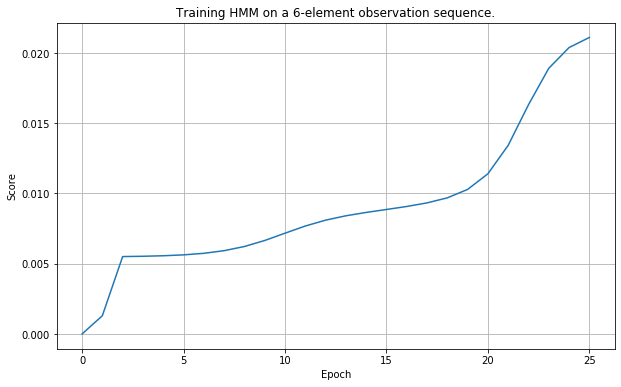
def train(self, observations: list, epochs: int, tol=None):
self._score_init = 0
self.score_history = (epochs + 1) * [0]
early_stopping = isinstance(tol, (int, float))
for epoch in range(1, epochs + 1):
score = self.update(observations)
print("Training... epoch = {} out of {}, score = {}.".format(epoch, epochs, score))
if early_stopping and abs(self._score_init - score) / score < tol:
print("Early stopping.")
break
self._score_init = score
self.score_history[epoch] = score
Example
1
2
3
4
5
6
7
8
9
10
11
np.random.seed(42)

observations = ['3L', '2M', '1S', '3L', '3L', '3L']

states = ['1H', '2C']
observables = ['1S', '2M', '3L']

hml = HiddenMarkovLayer.initialize(states, observables)
hmm = HiddenMarkovModel(hml)

hmm.train(observations, 25)
Verification
Let’s look at the generated sequences. The “demanded” sequence is:
| 0 | 1 | 2 | 3 | 4 | 5 | |
|---|---|---|---|---|---|---|
| 0 | 3L | 2M | 1S | 3L | 3L | 3L |
1
2
3
4
5
6
7
RUNS = 100000
T = 5

chains = RUNS * [0]
for i in range(len(chains)):
    chain = hmm.layer.run(T)[0]
    chains[i] = '-'.join(chain)
The table below summarizes simulated runs based on 100000 attempts (see above), with the frequency of occurrence and number of matching observations.
The bottom line is that if we have truly trained the model, we should see a strong tendency for it to generate us sequences that resemble the one we require. Let’s see if it happens.
1
2
3
4
5
6
7
8
9
10
11
df = pd.DataFrame(pd.Series(chains).value_counts(), columns=['counts']).reset_index().rename(columns={'index': 'chain'})
df = pd.merge(df, df['chain'].str.split('-', expand=True), left_index=True, right_index=True)

s = []
for i in range(T + 1):
    s.append(df.apply(lambda x: x[i] == observations[i], axis=1))

df['matched'] = pd.concat(s, axis=1).sum(axis=1)
df['counts'] = df['counts'] / RUNS * 100
df = df.drop(columns=['chain'])
df.head(30)
| counts | 0 | 1 | 2 | 3 | 4 | 5 | matched | |
|---|---|---|---|---|---|---|---|---|
| 0 | 8.907 | 3L | 3L | 3L | 3L | 3L | 3L | 4 |
| 1 | 4.422 | 3L | 2M | 3L | 3L | 3L | 3L | 5 |
| 2 | 4.286 | 1S | 3L | 3L | 3L | 3L | 3L | 3 |
| 3 | 4.284 | 3L | 3L | 3L | 3L | 3L | 2M | 3 |
| 4 | 4.278 | 3L | 3L | 3L | 2M | 3L | 3L | 3 |
| 5 | 4.227 | 3L | 3L | 1S | 3L | 3L | 3L | 5 |
| 6 | 4.179 | 3L | 3L | 3L | 3L | 1S | 3L | 3 |
| 7 | 2.179 | 3L | 2M | 3L | 2M | 3L | 3L | 4 |
| 8 | 2.173 | 3L | 2M | 3L | 3L | 1S | 3L | 4 |
| 9 | 2.165 | 1S | 3L | 1S | 3L | 3L | 3L | 4 |
| 10 | 2.147 | 3L | 2M | 3L | 3L | 3L | 2M | 4 |
| 11 | 2.136 | 3L | 3L | 3L | 2M | 3L | 2M | 2 |
| 12 | 2.121 | 3L | 2M | 1S | 3L | 3L | 3L | 6 |
| 13 | 2.111 | 1S | 3L | 3L | 2M | 3L | 3L | 2 |
| 14 | 2.1 | 1S | 2M | 3L | 3L | 3L | 3L | 4 |
| 15 | 2.075 | 3L | 3L | 3L | 2M | 1S | 3L | 2 |
| 16 | 2.05 | 1S | 3L | 3L | 3L | 3L | 2M | 2 |
| 17 | 2.04 | 3L | 3L | 1S | 3L | 3L | 2M | 4 |
| 18 | 2.038 | 3L | 3L | 1S | 2M | 3L | 3L | 4 |
| 19 | 2.022 | 3L | 3L | 1S | 3L | 1S | 3L | 4 |
| 20 | 2.008 | 1S | 3L | 3L | 3L | 1S | 3L | 2 |
| 21 | 1.955 | 3L | 3L | 3L | 3L | 1S | 2M | 2 |
| 22 | 1.079 | 1S | 2M | 3L | 2M | 3L | 3L | 3 |
| 23 | 1.077 | 1S | 2M | 3L | 3L | 3L | 2M | 3 |
| 24 | 1.075 | 3L | 2M | 1S | 2M | 3L | 3L | 5 |
| 25 | 1.064 | 1S | 2M | 1S | 3L | 3L | 3L | 5 |
| 26 | 1.052 | 1S | 2M | 3L | 3L | 1S | 3L | 3 |
| 27 | 1.048 | 3L | 2M | 3L | 2M | 1S | 3L | 3 |
| 28 | 1.032 | 1S | 3L | 1S | 2M | 3L | 3L | 3 |
| 29 | 1.024 | 1S | 3L | 1S | 3L | 1S | 3L | 3 |
And here are the sequences that we don’t want the model to create.
| counts | 0 | 1 | 2 | 3 | 4 | 5 | matched | |
|---|---|---|---|---|---|---|---|---|
| 266 | 0.001 | 1S | 1S | 3L | 3L | 2M | 2M | 1 |
| 267 | 0.001 | 1S | 2M | 2M | 3L | 2M | 2M | 2 |
| 268 | 0.001 | 3L | 1S | 1S | 3L | 1S | 1S | 3 |
| 269 | 0.001 | 3L | 3L | 3L | 1S | 2M | 2M | 1 |
| 270 | 0.001 | 3L | 1S | 3L | 1S | 1S | 3L | 2 |
| 271 | 0.001 | 1S | 3L | 2M | 1S | 1S | 3L | 1 |
| 272 | 0.001 | 3L | 2M | 2M | 3L | 3L | 1S | 4 |
| 273 | 0.001 | 1S | 3L | 3L | 1S | 1S | 1S | 0 |
| 274 | 0.001 | 3L | 1S | 2M | 2M | 1S | 2M | 1 |
| 275 | 0.001 | 3L | 3L | 2M | 1S | 3L | 2M | 2 |
As we can see, there is a tendency for our model to generate sequences that resemble the one we require, although the exact one (the one that matchs 6/6) places itself already at the 10th position! On the other hand, according to the table, the top 10 sequencies are still the ones that are somewhat similar to the one we request.
To ultimately verify the quality of our model, let’s plot the outcomes together with the frequency of occrence and compare it agains a freshly initialized model, which is supposed to give us completely random sequences - just to compare.
1
2
3
4
5
6
7
8
9
10
11
12
13
14
15
16
17
18
19
20
21
22
23
24
25
26
27
28
29
30
31
32
33
34
35
36
37
38
39
40
41
hml_rand = HiddenMarkovLayer.initialize(states, observables)
hmm_rand = HiddenMarkovModel(hml_rand)

RUNS = 100000
T = 5

chains_rand = RUNS * [0]
for i in range(len(chains_rand)):
    chain_rand = hmm_rand.layer.run(T)[0]
    chains_rand[i] = '-'.join(chain_rand)

df2 = pd.DataFrame(pd.Series(chains_rand).value_counts(), columns=['counts']).reset_index().rename(columns={'index': 'chain'})
df2 = pd.merge(df2, df2['chain'].str.split('-', expand=True), left_index=True, right_index=True)

s = []
for i in range(T + 1):
    s.append(df2.apply(lambda x: x[i] == observations[i], axis=1))

df2['matched'] = pd.concat(s, axis=1).sum(axis=1)
df2['counts'] = df2['counts'] / RUNS * 100
df2 = df2.drop(columns=['chain'])

fig, ax = plt.subplots(1, 1, figsize=(14, 6))

ax.plot(df['matched'], 'g:')
ax.plot(df2['matched'], 'k:')

ax.set_xlabel('Ordered index')
ax.set_ylabel('Matching observations')
ax.set_title('Verification on a 6-observation chain.')

ax2 = ax.twinx()
ax2.plot(df['counts'], 'r', lw=3)
ax2.plot(df2['counts'], 'k', lw=3)
ax2.set_ylabel('Frequency of occurrence [%]')

ax.legend(['trained', 'initialized'])
ax2.legend(['trained', 'initialized'])

plt.grid()
plt.show()
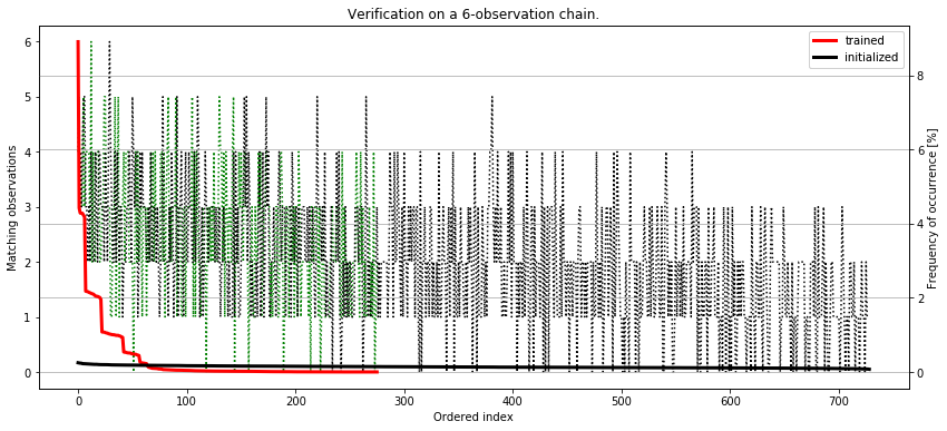
It seems we have successfully implemented the training procedure. If we look at the curves, the initialized-only model generates observation sequences with almost equal probability. It’s completely random. However, the trained model gives sequences that are highly similar to the one we desire with much higher frequency. Despite the genuine sequence gets created in only 2% of total runs, the other similar sequences get generated approximately as often.
Conclusion
In this article, we have presented a step-by-step implementation of the Hidden Markov Model. We have created the code by adapting the first principles approach. More specifically, we have shown how the probabilistic concepts that are expressed through eqiations can be implemented as objects and methods. Finally, we demonstrated the usage of the model with finding the score, uncovering of the latent variable chain and applied the training procedure.
Do you want more?
- Check out my “Python Data Science Algorithm Gallery” project on Github.
- The code for this project is also stored as “Markeasy” library.
- Take a look at the “Morning Insanity” article, where we are putting this code into practice for higher good ;).