Multi-Layer Perceptron & Backpropagation - Implemented from scratch

Oct 26, 2020

Introduction

Writing a custom implementation of a popular algorithm can be compared to playing a musical standard. For as long as the code reflects upon the equations, the functionality remains unchanged. It is, indeed, just like playing from notes. However, it lets you master your tools and practice your ability to hear and think.

In this post, we are going to re-play the classic Multi-Layer Perceptron. Most importantly, we will play the solo called backpropagation, which is, indeed, one of the machine-learning standards.

As usual, we are going to show how the math translates into code. In other words, we will take the notes (equations) and play them using bare-bone numpy.

FYI: Feel free to check another “implemented from scratch” article on Hidden Markov Models here.

Overture - A Dense Layer

Data

Let our (most generic) data be described as pairs of question-answer examples: $(\mathbf{x}^{(i)}, y^{(i)})$ , where $\mathbf{X} \in \mathbb{R}^{m \times n}$ is as a matrix of feature vectors, $\mathbf{y} \in \mathbb{R}^m$ is known a matrix of labels and $i$ refers to an index of a particular data example. Here, by $n$ we understand the number of features and $m$ is the number of examples, so $i \in \{1, 2, \cdots, m\}$ . Also, we assume that $y^{(i)} \in \{0, 1\}$ thus posing a binary classification problem for us. Here, it is important to mention that the approach won’t be much different if $y$ was a multi-class or a continuous variable (regression).

To generate the mock for the data, we use the sklearn’s make_classification function.

1
2
3
4
5
6
7
import numpy as np
from sklearn.datasets import make_classification

np.random.seed(42)
X, y = make_classification(n_samples=10, n_features=4, 
    n_classes=2, n_clusters_per_class=1)
y_true = y.reshape(-1, 1)

Note that we do not split the data into the training and test datasets, as our goal would be to construct the network. Therefore, if the model overfits it would be a perfect sign!

At this stage, we adopt the convention that axis=0 shall refer to the examples $i$ , while axis=1 will be reserved for the features $j \in \{1, 2, \cdots, n\}$ . Naturally, for binary classification $\dim \mathbf{y} = (m, 1)$ .

A single perceptron

Figure 1. shows the concept of a single perceptron for the sake of showing the notation.

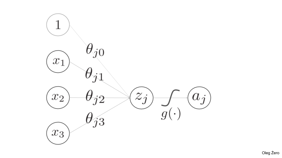
/assets/mlp-backpropagation/figure1.png — Figure 1. A single perceptron.

The coefficients $\theta_{jj'}$ are known as weights and we can group them with a matrix $\mathbf{\Theta}$ . The indices denote that we map an input feature $j'$ to an output feature $j$ . We also introduce a bias term $x_0 = 1$ , and therefore we can calculate $z_j$ using a single vector-matrix multiplication operation, starting from $j' = 0$ :

$z_j = \sum_{j' = 0}^n \theta_{jj'} x_{j'}$

that can be written in a compact form:

$\mathbf{z} = \mathbf{\Theta}^T \mathbf{x}.$

This way we also don’t discriminate between the weight terms $\mathbf{W}$ and bias terms $\mathbf{b}$ . Everything becomes $\mathbf{\Theta} \equiv \mathbf{W}$ .

Next, the output of the inner product is fed to a non-linear function $g(\cdot)$ , known as the activation function.

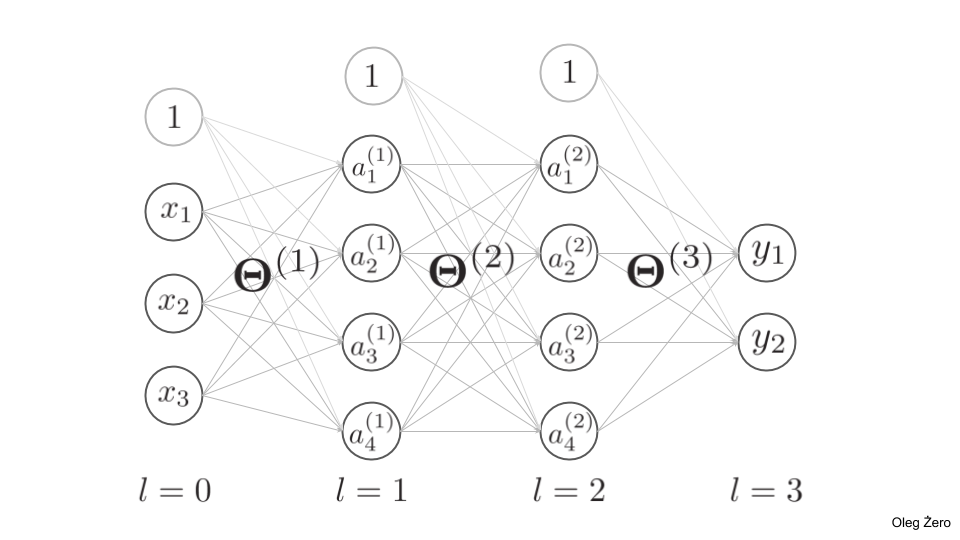
The strength of neural networks lies in the “daisy-chaining” of layers of these perceptrons. Therefore, we can describe the whole network with a non-linear transformation that uses these two equations combined. Recursively, we can write that for each layer $l$

$\mathbf{a}^{(l)} = g(\mathbf{\Theta}^T\mathbf{a}^{(l - 1)}),$

with $\mathbf{a}^{(0)} = \mathbf{x}$ being the input and $\hat{\mathbf{y}} = \mathbf{a}^{(L)}$ being the output.

Figure 2. shows an example architecture of a multi-layer perceptron.

/assets/mlp-backpropagation/figure2.png — Figure 2. A multi-layer perceptron, where `L = 3`. In the case of a regression problem, the output would not be applied to an activation function. Apart from that, note that every activation function needs to be non-linear. Otherwise, the whole network would collapse to linear transformation itself thus failing to serve its purpose.

The code

Having the equations written down, let’s wrap them up with some code.

First of all, as the layer formula is recursive, it makes total sense to discriminate a layer to be an entity. Therefore, we make it a class:

1
2
3
4
5
6
7
8
9
10
11
12
13
14
15
16
17
18
19
20
21
22
23
24
25
26
27
28
29
30
31
32
class DenseLayer:
    def __init__(
            self, 
            n_units, 
            input_size=None, 
            activation=None, 
            name=None):self.n_units = n_units
        self.input_size = input_size
        self.W = None
        self.name = name
        self.A = None
        
        self.activation = activation
        self.fn, self.df = self._select_activation_fn(activation)

    def __repr__(self):
        return f"Dense['{self.name}'] in:{self.input_size} + 1, out:{self.n_units}"

    def init_weights(self):
        self.W = np.random.randn(self.n_units, self.input_size + 1)

    @property
    def shape(self):
        return self.W.shape

    def __call__(self, X):
        m_examples = X.shape[0]
        X_extended = np.hstack([np.ones((m_examples, 1)), X])
        Z = X_extended @ self.W.T
        A = self.fn(Z)
        self.A = A
        return A

OK. Let’s break it down…

First of all, all we need to know about a layer is the number of units and the input size. However, as the input size will be dictated by either the data matrix $\mathbf{X}$ or the size of the preceding layer, we will leave this parameter as optional. This is also the reason, why we leave the weights’ initialization step aside.

Secondly, both the __repr__ method as well as the self.name attribute serves no other purpose but to help us to debug this thing. Similarly, the shape property is nothing, but a utility.

The real magic happens within the __call__ method that implements the very math we discussed so far. To to have the calculations vectorized, we prepare the layer to accept whole arrays of data. Naturally, we associate the example count $m$ with the 0th axis, and the features’ count $n$ with the 1st axis. Once the layer accepts it, it extends the array with a whole column of 1’s to account for the bias term $x_0$ . Next, we perform the inner product, ensuring that the output dimension will match (m_examples, n_units). Finally, we apply a particular type of a non-linear transformation known as sigmoid (for now):

$g(z) = \frac{1}{1 + e^{-z}}.$

Forward propagation

Our “dense” layer (a layer perceptrons) is now defined. It is time to combine several of these layers into a model.

1
2
3
4
5
6
7
8
9
10
11
12
13
14
15
16
17
18
19
20
21
22
23
24
class SequentialModel:
    def __init__(self, layers, lr=0.01):
        input_size = layers[0].n_units
        layers[0].init_weights()
        for layer in layers[1:]:
            layer.input_size = input_size
            input_size = layer.n_units
            layer.init_weights()
        self.layers = layers

    def __repr__(self):
        return f"SequentialModel n_layer: {len(self.layers)}"

    def forward(self, X):
        out = self.layers[0](X)
        for layer in self.layers[1:]:
            out = layer(out)
        return out

    @staticmethod
    def cost(y_pred, y_true):
        cost = -y_true * np.log(y_pred) \
               - (1 - y_true) * np.log(1 - y_pred)
        return cost.mean()

The whole constructor of this class is all about making sure that all layers are initialized and “size-compatible”. The real computations happen in the .forward() method and the only reason for the method to be called this way (not __call__) is so that we can create twin method .backward once we move on to discussing the backpropagation.

Next, the .cost method implements the so-called binary cross-entropy equation that firs our particular case:

$J(\mathbf{\Theta}) = \frac{-1}{m}\sum_{i = 1}^m \left( \mathbf{y} \ln \hat{\mathbf{y}}) + (1 - \mathbf{y}) \ln (1 - \hat{\mathbf{y}}) \right)$

If we went down with a multi-class classification or regression, this equation would have to be replaced.

Finally, the __repr__ method exists only for the sake of debugging.

Instantiation

These two classes are enough to make the first predictions!

1
2
3
4
5
6
7
8
9
10
11
12
np.random.seed(42)

model = SequentialModel([
    DenseLayer(6, input_size=X.shape[1], name='input'),
    DenseLayer(4, name='1st hidden'),
    DenseLayer(3, name='2nd hidden'),
    DenseLayer(1, name='output')
])

y_pred = model.forward(X)
model.cost(y_pred, y_true)
>>> 0.8305111958397594

That’s it! If done correctly, we should see the result.

The only problem is, of course, that the result is completely random. After all, the network needs to be trained. Therefore, to make it trainable will be our next goal.

Back-propagation

There exist multiple ways to train a neural net, one of which is to use the so-called normal equation

$\mathbf{\Theta} = (\mathbf{X}^T\mathbf{X})^{-1}\mathbf{X}^T\mathbf{y}.$

Another option is to use an optimization algorithm such as Gradient Descent, which is an iterative process to update weight is such a way, that the cost function associated with the problem is subsequently minimized:

$\mathbf{\Theta} = \arg \min_{\Theta} J(\mathbf{\Theta)}.$

To get to the point, where we can find the most optimal weights, we need to be able to calculate the gradient of $J$ . Only then, we can expect to be altering $\mathbf{\Theta}$ in a way that would lead to improvement. Consequently, we need to incorporate this logic into our model.

Let’s take a look at the equations, first.

Dependencies and the chain-rule

Thinking of $J$ as a function of predictions $\hat{\mathbf{y}}$ , we know it has implicit dependencies on every weight $\theta_{jj'}^{(l)}$ . To get the gradient, we need to resolve all the derivatives of $J$ with respect to every possible weight. Since the dependency is dictated by the architecture of the network, to resolve these dependencies we can apply the so-called chain rule. In other words, to get the derivatives $\frac{\partial J}{\partial \theta_{jj'}^{(l)}}$ , we need to trace back “what depends on what”.

Here is how it is done.

Let’s start with calculating the derivative of the cost function with respect to some weight $\theta_{jj'}^{(l)}$ . To make the approach generic, irrespectively from if our problem is a classification or a regression type problem, we can estimate a fractional error that the network commits at every layer as a squared difference between the activation values $a_{j}^{(l)}$ and a respective local target value $t_j^{(l)}$ , which is what the network would achieve at the nodes if it was perfect. Therefore,

$E^{(l)} = \frac{1}{2}\sum_{j = 1}^{n_{l}} (a_j^{(l)} - t_j^{(l)})^2$

Now, to find a given weight’s contribution to the overall error for a given layer $l$ , we calculate $\frac{\partial E}{\partial \theta_{jj'}^{(l)}}$ . Knowing that when going “forward”, we have $a^{(l)}$ dependents on $z$ through an activation function $g$ , whose argument in turns depends on contributions from the previous layers, we apply the chain-rule:

$\Delta_{jj'}^{(l)} = \frac{\partial E^{(l)}}{\partial a_j} \frac{\partial a_j}{\partial z_j} \frac{\partial z_j}{\partial \theta_{jj'}^{(l)}}.$

Partial error function derivative

Now, let’s break it down. The first term gives the following contribution:

$\frac{\partial E}{\partial a_j} = a_j - t_j.$

Activation function derivative

Next, the middle term depends on the actual choice of the activation function. For the sigmoid function, we have:

$\frac{\partial a_j}{\partial z_j} = \frac{\partial g(z_j)}{\partial z_j} = \frac{e^{-z_j}}{(1 + e^{-z_j})^2},$

which we can rewrite as $g(z_j)(1 - g(z_j))$ .

Similarly, for other popular activation function, we have

$\frac{\partial}{\partial z_j} \tanh(z_j) = 1 - \tanh^2(z_j), \\ \frac{\partial}{\partial z_j} \text{ReLU}(z_j) = \left\{\begin{matrix}0 \text{ if } z_j < 0 \\ 1 \text{ if } z_j \ge 0\end{matrix}\right. .$

Note that although the ReLU function is not differentiable, we can calculate its “quasiderivative”, since we will only ever be interested in its value at a given point.

Previous layer

Finally, the dependency on the previous layer. We know that $z_j^{(l)} = (\Theta_{j}^{(l)})^T \mathbf{a}^{(l - 1)}$ . Hence, the derivative is simply:

$\frac{\partial z_j}{\partial \theta_{jj'}^{(l)}} = a_{j'}^{(l - 1)}.$

Unless we consider the first layer, in which case $a_{j'} \equiv x_{j'}$ , we can expect further dependency of this activation on other weights and the chain-rule continues. However, at a level of a single layer, we are only interested in the contribution of each of its nodes to the global cost function, which is the optimization target.

Collecting the results together, the contribution to each layer becomes:

$\Delta_{jj'}^{(l)} = ((a^{(l)}_j - t^{(l)}_j)g'(z_j^{(l)})) \cdot a_{j'}^{(l - 1)} = \delta_j^{(l)} \cdot a_{j'}^{(l - 1)},$

where $\delta$ ’s can be thought of as indicators of how far we deviate from the optimal performance.

This quantity, we need to pass on “backward” through the layers, starting from $l = L$ :

$\delta^{(L)} = \hat{\mathbf{y}} - \mathbf{y}$

Then going recursively:

$\delta_{j'}^{(l - 1)} = \sum_j \theta_{jj'}^{(l)} (a_j^{(l)} - t_j^{(l)}) g'(z_j^{(l)}),$

which may be expressed as: $\delta^{(l - 1)} = ((\mathbf{\Theta}^{(l)})^T \cdot \delta^{(l)}) g'(\mathbf{z})$ , until we reach $\delta^{(0)} = \mathbf{x} - \mathbf{t}^{(0)} = 0$ , as there is no “shift” between the data and the data iteself.

Implementation of the backpropagation

This is all we need! Looking carefully at the equations above, we can note three things:

It provides us with an exact recipe for defining how much we need to alter each weight in the network.
It is recursive (just defined “backward”), hence we can re-use our “layered” approach to compute it.
It requires $a$ ’s at every layer. However, since these are quantities are calculated when propagating forward, we can cache them.

In addition to that, since we know how to handle different activation functions, let us also incorporate them into our model.

Different activation functions

Probably the cleanest way to account for the different activation functions would be to organize them as a separate library. However, we are not developing a framework here. Therefore, we will limit ourselves to updating the DenseLayer class:

1
2
3
4
5
6
7
8
9
10
11
12
13
14
15
16
17
18
19
20
21
22
23
24
25
26
27
28
29
30
31
32
33
class DenseLayer:
    def __init__(self, n_units, 
        input_size=None, activation='sigmoid', name=None):
        
        self.n_units = n_units
        self.input_size = input_size
        self.W = None
        self.name = name
        self.A = None  # here we will cache the activation values
        self.fn, self.df = self._select_activation_fn(activation)

    def _select_activation_fn(self, activation):
        if activation == 'relu':
            fn = lambda x: np.where(x < 0, 0.0, x)
            df = lambda x: np.where(x < 0, 0.0, 1.0)
        elif activation == 'sigmoid':
            fn = lambda x: 1 / (1 + np.exp(-x))
            df = lambda x: x * (1 - x)
        elif activation == 'tanh':
            fn = lambda x: (np.exp(x) - np.exp(-1)) / (np.exp(x) + np.exp(-x))
            df = lambda x: 1 - x**2
        elif activation is None:
            fn = lambda x: x
            df = lambda x: 1.0
        else:
            NotImplementedError(f"Function {activation} cannot be used.")
        return fn, df

    def __call__(self, X):
        ...  # as before
        A = self.fn(Z)
        self.A = A
        return A

With caching $a$ and different activation functions being supported, we can move on to defining the .backprop method.

Passing on delta

Again, let’s update the class:

1
2
3
4
5
6
class DenseLayer:
    ...  # as before

    def backprop(self, delta, a):
        da = self.df(a)  # the derivative of the activation fn
        return (delta @ self.W)[:, 1:] * da

Here is where $\delta$ s is being passed down through the layers. Observe that we “trim” the $\delta$ matrix by eliminating $\delta_{j = 0}$ , which relate to the bias terms.

Updating weights

Updating of $\theta$ ’s needs to happen at the level of the model itself. Having the right behavior at the level of a layer, we are ready to add this functionality to the SequentialModel class.

1
2
3
4
5
6
7
8
9
10
11
12
13
14
15
16
17
18
19
20
21
22
class SequentialModel:
    ...  # as before

    def _extend(self, vec):
        return np.hstack([np.ones((vec.shape[0], 1)), vec])

    def backward(self, X, y_pred, y_true):
        n_layers = len(self.layers)
        delta = y_pred - y_true
        a = y_pred

        dWs = {}
        for i in range(-1, -len(self.layers), -1):
            a = self.layers[i - 1].A

            dWs[i] = delta.T @ self._extend(a)
            delta = self.layers[i].backprop(delta, a)

        dWs[-n_layers] = delta.T @ self._extend(X)

        for k, dW in dWs.items():
            self.layers[k].W -= self.lr * dW

The loop index runs back across the layers, getting delta to be computed by each layer and feeding it to the next (previous) one. The matrices of the derivatives $\Delta^{(l)}$ (or dW) are collected and used to update the weights at the end. Again, the ._extent() method was used for convenience.

Finally, note the differences in shapes between the formulae we derived and their actual implementation. This is, again, the consequence of adopting the convention, where we use the 0th axis for the example count.

Time for training!

We have finally arrived at the point, where we can take advantage of the methods we created and begin to train the network. All we need to do is to instantiate the model and let it call the .forward() and .backward() methods interchangeably until we reach convergence.

1
2
3
4
5
6
7
8
9
10
11
12
13
np.random.seed(42)

N = X.shape[1]
model = SequentialModel([
    DenseLayer(6, activation='sigmoid', input_size=N, name='input'),
    DenseLayer(4, activation='tanh', name='1st hidden'),
    DenseLayer(3, activation='relu', name='2nd hidden'),
    DenseLayer(1, activation='sigmoid', name='output')
])

for e in range(100):
    y_pred = model.forward(X)
    model.backward(X, y_pred, y_true)

The table below presents the result:

example	predicted	true
0	0.041729	0.0
1	0.042288	0.0
2	0.951919	1.0
3	0.953927	1.0
4	0.814978	1.0
5	0.036855	0.0
6	0.228409	0.0
7	0.953930	1.0
8	0.050531	0.0
9	0.953687	1.0

Conclusion

It seems our network indeed learned something. More importantly, we have shown how mathematical equations can also suggest more reasonable ways to implement them. Indeed, if you look carefully, you can perhaps notice that this implementation is quite “Keras-like”.

This is not a coincidence. The reason for this to happen is the fact it the very nature of the equations we used. As the concept uses the concept of derivatives, we follow the “chain-rule” also in the programming, which applies to other types of layers as well, and it the reason why Tensorflow or PyTorch organize the equations as graphs using a symbolic math approach. Although the intention of this work was never to compete against these well-established frameworks, it hopefully makes them more intuitive.

Coming back to the beginning, we hope that you liked the “melody” of these equations played using bare-bone numpy. If you did, feel encouraged to read our previous “implemented from scratch” article on Hidden Markov Models here.