How to handle autoregressive model over multiple time series?

Introduction

Autoregressive models are among the “more difficult” to implement when it comes to data preparation. As the models are expected to yield daily or hourly predictions, the datasets themselves are expected to grow and expand with every new observation requiring the models to undergo regular retraining. Consequently, handling the data becomes a highly dynamic process where one has to be extra careful to ensure that no data leakage is present at any given point.

Surprisingly, but unfortunately, most tutorials on autoregression put way more emphasis on the models and algorithms, while not focusing that much on the data preparation side of things. Since their goal is to explain the autoregression concept (and they do it so well, for example: Machine Learning Mastery or article 1, article 2 from Towards Data Science), handing of the data preparation is limited to a single uni- or multi-variate time series. Tensorflow.org provides a more extensive explanation, although their approach is not easily extendable to cases of multiple multi-variate time series.

In this article, I would like to show you, how you can take advantage of the factory pattern to encapsulate the logic at various levels of abstraction without losing the flexibility in your code. For demonstration, I will use the same dataset (Jena Climate Dataset) as used in the Tensorflow’s tutorial. However, to complicate the matter a bit, I will create a few copies of the data with random perturbations to mimic a situation where our model’s task is to predict the weather at several geo-locations. Also, it is not uncommon to see time series datasets containing observations that “come and go” in random intervals. To gain as many training examples from the dataset as possible, I will also account for this fact.

Making the data a bit more realistic…

For simplicity, I will skip the part that deals with the feature generation and focus on the T (degC) column. Let’s assume that our model’s task would be to predict the mean temperatures in several cities given first, last, min, and max temperature. Naturally, you could extend the same reasoning to all the columns in the dataset or choose a different target (e.g. predicting the mean temperature from the past mean temperatures). It’s all up to you. What I focus on here, however, is to build the training examples from multiple multi-dimensional series with special care for avoiding data leakage and “production-like” nature where new observations are expected to come each day.

Fetching data

Let’s begin with fetching the data and resampling it to daily intervals.

1
2
3
4
5
6
7
8
9
10
11
12
13
14
15
16
17
18
19
20
import numpy as np
import pandas as pd
import tensorflow as tf


zip_path = tf.keras.utils.get_file(
    origin="https://storage.googleapis.com/tensorflow/tf-keras-datasets/jena_climate_2009_2016.csv.zip",
    fname="jena_climate_2009_2016.csv.zip",
    extract=True,
)
csv_path, _ = os.path.splitext(zip_path)

df = pd.read_csv(csv_path) \
    .assign(date=lambda x: pd.to_datetime(x["Date Time"])) \
    .set_index("date") \
    .get(["T (degC)"]) \
    .resample("D") \
    .aggregate(["first", "last", "min", "max", "mean"])

df.columns = [c[1] for c in df.columns]

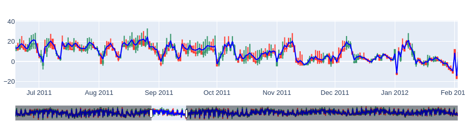
Having created the [first, last, min, max] columns, let’s use the candlestick to display the data.

✕

Figure 1.

The candles represent the daily variations to the temperature. The blue line depicts the mean temperature, which we understand as our target.

Mocking the case

Now, it’s time to mock a more realistic scenario in which the data availability is not ideal.

1
2
3
4
5
6
7
8
9
10
11
12
13
14
15
16
17
18
19
np.random.seed(42)

CITIES = [
    "London", "Oslo", "Warsaw", "Copenhagen", "Amsterdam", "Dublin",
    "Brussels", "Stockholm", "Prague", "Paris", "Rome", "Budapest",
    "Lisbon", "Vienna", "Madrid", "Riga", "Berlin", "Belgrade", "Sofia",
]

series = {}
for city in CITIES:
    X = df.copy()
    X += 0.75 * X.std() * np.random.randn()

    bounds = np.random.randint(0, len(X), size=2)
    bounds = sorted(bounds)
    slc = slice(*bounds)
    X = X.iloc[slc]

    series[city] = X

After this… modification, our data looks like this:

✕

Figure 2.

The heatmap displays the target value, which is the mean temperature.

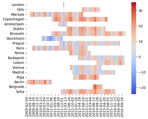
Isn’t that more how data behaves in reality? As you can see, depending on the city, our availability is different. Especially for London, our choices for the sequences’ lengths may be limited.

Generating samples

In autoregression, it is a common approach to use a rolling window that would slide along the time dimension and divide it into history and future sub-sequences. As the window moves forward (here, with a step size of one day), each time a new (X, y) pair is obtained. These pairs are then fed into the model for training.

When defining windows two considerations need to be taken into account. First of all, the history part of the window must never enter time regions where data is not supposed to yet be observed. Otherwise, data leakage is more than guaranteed! Conversely, the future part of the window can enter them. However, for the training, validation, and test subsets, we should ensure that the data exists so that predicted values can be compared with true values. During the inference, it is different. Technically, it is not possible to observe tomorrow’s numbers today. But as the sun raises again, we can compare the predictions.

Secondly, the time “horizon” is going to constantly shift forward. For models’ training, this means our historical dataset grows and so should the time horizons be pushed to the future as well.

As you can see, the whole situation is quite dynamic. Unless designed with sense, the code can quickly lose transparency and lead to errors.

Solution

The key to solving the problem is to delegate responsibility to different classes. For example, splitting the series into training and testing parts should not be a part of the rolling window logic. Similarly, once the window is rolling it is only supposed to generate data samples without needing to care about the dates.

Thinking about it, we can discriminate the following chain of responsibilities.

1. First, it is useful to have some configuration file(s) that will store the parameters. Usually, I would have two separate files such as development.ini, and production.ini and a get_config function.
2. Once the constants are loaded, let’s use a TimeSplitter class to calculate time intervals and give us boundary dates. These dates will define the beginning and the end of the training, test, and validation parts.
3. The dates essentially tell where the rolling windows are supposed to operate. However, as mentioned earlier, we don’t want them to manage the time. The rolling windows are only going to generate samples, and this is where the factory pattern comes in. Let’s have a WindowFactory class to consume the boundaries and create Window objects.
4. Finally, depending on the need, we may construct different kinds of Windows (e.g. with or without a stepsize, an averaging window, etc.). Still, once the factory class has translated the dates into indices, each Window is only going to be given a time series chunk to roll over and generate the (X, y)-pairs.

Constants

Before we begin, let’s agree on a few parameters.

development.ini

1
2
3
4
5
6
[constants]
horizon = 2022-02-28
test_split_days = 30
val_split_days = 90
history_days = 21
future_days = 7

To clarify the convention: horizon defines the ultimate “blinding” of the dataset. It is supposed be “today”, beyond which no observation exists yet. In production, this parameter is expected to be updated daily. Then, the training, validation, and test sets are defined over the intervals $t_\text{training} \in [-\infty, h - 91], t_\text{validation} \in [h - 90, h - 31]$ and $t_\text{test} \in [h - 30, h]$, respectively. Finally, in this scenario, Windows are expected to support models that render predictions 7 days into the future, knowing the last 21 days.

I will leave implementing get_config… Once we read the data, the next step is:

Time Splitter

1
2
3
4
5
6
7
8
9
10
11
12
13
14
15
16
17
18
19
20
21
22
23
24
25
26
27
28
29
30
31
32
33
34
35
36
37
38
39
40
41
42
43
44
45
46
47
48
49
50
51
52
53
54
55
56
57
from typing import Optional, Text, Tuple, TypeVar

import pandas as pd

TS = TypeVar("TS")


class TimeSplitter:
    def __init__(
        self,
        horizon: Text,
        val_split_days: int,
        test_split_days: int,
        history_days: int,
        future_days: int,
    ) -> TS:
        self.horizon = pd.Timestamp(horizon)
        self.val_split_days = pd.Timedelta(val_split_days, unit="days")
        self.test_split_days = pd.Timedelta(test_split_days, unit="days")
        self.history_days = pd.Timedelta(history_days, unit="days")
        self.future_days = pd.Timedelta(future_days, unit="days")

        # here you can put additional assertion logic such as non-negative days, etc.

    @property
    def _test_upto(self) -> pd.Timestamp:
        return self.horizon

    @property
    def _test_from(self) -> pd.Timestamp:
        return self.horizon - self.test_split_days - self.history_days

    @property
    def _validation_upto(self) -> pd.Timestamp:
        return self.horizon - self.test_split_days - pd.Timedelta(1, unit="days")

    @property
    def _validation_from(self) -> pd.Timestamp:
        return self.horizon - self.val_split_days - self.history_days

    @property
    def _train_upto(self) -> pd.Timestamp:
        return self.horizon - self.val_split_days - pd.Timedelta(1, unit="days")

    @property
    def _train_from(self) -> None:
        return None  # defined only for consistency

    def get_boundaries(self, subset: Optional[Text] = "training") -> Tuple[pd.Timestamp]:
        if subset == "training":
            return self._train_from, self.train_upto
        elif subset == "validation":
            return self._validation_from, self._validation_upto
        elif subset == "test":
            return self._test_from, self._test_upto
        else:
            raise NotImplementedError(f"Requested subset '{subset}' is not supported.")

As mentioned earlier, the only goal of the TimeSplitter is to figure out the boundaries. With additional logic, we can introduce assertions, warnings, or errors against situations resulting in ill-conditioned results. Also, we could replace the if-else statement with an Enum class, limiting the choices to only a few predefined options. This would go a bit beyond the scope of this article, so let’s move on to implementing the factory class.

Window Factory

Now, it is time for the factory class. Once the date time boundaries are calculated, we expect the class to use the information to trim the series and spawn the window.

1
2
3
4
5
6
7
8
9
10
11
12
13
14
15
16
17
18
19
20
21
22
23
24
25
26
27
28
29
30
31
32
33
34
35
36
37
class WindowFactory:
    def __init__(
        self,
        history_days: int,
        future_days: int,
        first_allowed_date: Optional[pd.Timestamp] = None,
        last_allowed_date: Optional[pd.Timestamp] = None,
    ) -> WF:
        self.hdays = history_days
        self.fdays = future_days
        self.lower_date = first_allowed_date
        self.upper_date = last_allowed_date

    def __repr__(self) -> Text:
        lower = self.lower_date or "-inf"
        upper = self.upper_date or "+inf"
        interval = f"['{lower}':'{upper}']"
        shape = f"({self.hdays}, {self.fdays})"
        name = self.__class__.__name__

        return f"{name}(interval={interval}, shape={shape})"

    def create(self, df: pd.DataFrame) -> Optional[W]:
        t0 = self.lower_date if self.lower_date is pd.NaT else None
        t1 = self.upper_date if self.upper_date is pd.NaT else None
        slc = slice(t0, t1)
        chunk = df.loc[slc]

        if (width := self.hdays + self.fdays) > len(chunk):
            print(f"Not possible to spawn a window of width={width}.")
            return None

        return Window(
            chunk,
            history_days=self.hdays,
            future_days=self.fdays,
        )

There are several ways to implement the class. The core functionality is provided by the .create method. It expects a time series as a pd.DataFrame and its goal is to correctly slice the input data. Here, we take advantage of the fact that indices in our dataframes are pd.DateTimeIndex objects. However, if we worked with plain numpy, the idea would be the same.

The method can also be extended to support different kinds of windows if needed. In our version, we use only one type of Window, so no other input arguments are necessary.

Finally, we introduce the __repr__ method to display the “capability” of the factory in terms of the interval and window shape. It is purely for the sake of debugging and readability.

The Window

So how is the Window going to be defined? After all, the date time and indexing management are already done, all we need is an object that produces samples.

1
2
3
4
5
6
7
8
9
10
11
12
13
14
15
16
17
18
19
20
21
22
23
24
25
26
27
28
29
30
31
W = TypeVar("W")

class Window:
    def __init__(
        self,
        chunk: pd.DataFrame,
        history_days: int,
        future_days: int,
    ) -> W:
        self.X = chunk.to_numpy()
        self.hdays = history_days
        self.fdays = future_days

    @property
    def width(self) -> int:
        return self.hdays + self.fdays

    def __len__(self) -> int:
        return len(self.X) - self.width + 1

    def __repr__(self) -> Text:
        name = self.__class__.__name__
        iters = f"iters: {len(iters)}"

        return f"{name}[{iters}]({self.hdays, self.fdays)"

    def get_generator(self) -> Generator[np.ndarray, None, None]:
        for idx in range(len(self)):
            slc = slice(idx, idx + self.width)

            yield self.X[slc]

The .get_generator method is self-explanatory. It gives off slices of the time series by rolling along the time dimension with a step size of one day. Here, the __len__ method is used to express the number of samples the Window will produce. For example, if the series contains 5 records, and the window’s width is 2, it should roll exactly 4 times (hence + 1 in the end).

But wait!

The generator does not yield (X, y)-pairs, right? Correct.

Formulating pairs is easy, though. With slight modification, we can redefine the generator method:

1
2
3
4
5
6
def get_sample_pairs(self) -> Generator[np.ndarray, None, None]:
    for idx in range(len(self)):
        slc_X = slice(idx, idx + self.hdays)
        slc_y = slice(idx + self.hdays, idx + self.width)

        yield (self.X[slc_X, :4], self.X[slc_y, -1])

tf.data version

If you choose to work with Keras, however, you may find it useful to replace the generator with tf.data.Dataset object that contains the pair inside and pass that into the model. To achieve that, let’s make the Window object callable by adding one more method.

1
2
3
4
5
6
7
8
9
10
11
12
13
14
15
16
17
    def __call__(self) -> tf.data.Dataset:
        generator = lambda: self.get_generator()
        signature = tf.TensorSpec(
            shape=(self.width, 5),
            dtype=tf.float32,
            name=self.__class__.__name__,
        )
        ds = tf.data.Dataset.from_generator(
            generator,
            output_signature=signature,
        )
        ds = ds.map(lambda tensor: [
            tensor[:self.hdays, :4],
            tensor[self.hdays:self.width, -1:],
        ])

        return ds

The downside of using this method is the fact that we create a lazy loading mechanism, just to consume the data eagerly. On the other hand, using tf.data provides us with a lot of useful functions (e.g. prefetch, shuffle, batch or concatenate), which makes the data easier to handle later.

The whole flow

Let’s revisit our solution and create the full training, test, and validation datasets with help of the implemented logic.

1
2
3
4
5
6
7
8
9
10
11
12
13
14
15
16
17
18
19
20
21
22
23
24
25
26
27
28
29
30
31
32
33
34
35
36
37
38
39
40
41
42
43
44
45
46
47
48
49
50
51
52
53
54
# from config...
horizon = "2014-01-01"
test_split_days = 30
val_split_days = 90
history_days = 21
future_days = 7


def get_window_factory(splitter, name):
    bounds = splitter.get_boundaries(name)

    return WindowFactory(
        history_days=history_days,
        future_days=future_days,
        first_allowed_observation_date=bounds[0],
        last_allowed_observation_date=bounds[1],
    )


def get_dataset(factory, series):
    windows = {}
    for city, X in series.items():
        window = factory.create(X)
        if window is None:
            print("City skipped:", city)
            continue
    
        windows[city] = window
   
    _, window = windows.popitem()
    ds = window()
    for window in windows.values():
        _ds = window()
        ds = ds.concatenate(_ds)
    
    return ds


if __name__ == "__main__":
    splitter = TimeSplitter(
        horizon=horizon,
        test_split_days=test_split_days,
        val_split_days=val_split_days,
        history_days=21,
        future_days=7,
    )

    training_factory = get_window_factory(splitter, "training")
    validation_factory = get_window_factory(splitter, "validation")
    test_factory = get_window_factory(splitter, "test")
    
    ds_train = get_dataset(training_factory, series)
    df_val = get_dataset(validation_factory, series)
    df_test = get_dataset(test_factory, series)

Conclusions

And this is it! Once we have loaded the constants and split the dates using TimeSplitter, we create three factories for each dataset respectively. The samples are then generated and collected using tf.data.Datasets objects. However we choose to parametrize the code, the process stays the same, although if the datasets are too narrow (or the Window’s width too large), we may end up having only a few samples.

To verify the approach, you can assert the total number of samples.

1
2
3
4
count_1 = len([x for x in ds.as_numpy_iterator()])
count_2 = sum([len(w) for w in windows.values()])

assert count_1 == count_2

This code can certainly be improved. However, as you can see, this approach is simple to use and the code should be easy to maintain. It is also adaptable to any generic multivariate time series. It all depends on how you envision the (X, y)-pairs to look like (e.g. scalars, vectors, tensors, …)? Still, by applying this simple pattern, you can almost completely separate the data preparation code from the actual model, allowing you to iterate quickly over your ideas without worrying about data leakage to creeping up in your results.