Restoring intuition over multi-dimensional space

Feb 16, 2020

Introduction

We would not be human if we did not curse things. As beings that are confined in a three-dimensional world, we tend to blame space whenever we have a problem to visualize data that extend to more than three dimensions. From scientific books and journal papers to simple blog articles and comments the term: “curse of dimensionality” is being repeated like a mantra, almost convincing us that any object, whose nature extends to something more than just “3D” is out of reach to our brains.

This article is going to discuss neither data visualization nor seek to conform to the common opinion that highly-dimensional space is incomprehensible.

Quite opposite: the highly-dimensional space is not incomprehensible. It is just weird and less intuitive. Fortunately, take advantage of some mathematical tools and use them as a “free ticket” to gain more intuition. More precisely, we will present three “routes” we can use to get a better feeling on how things play out in “ND space.”

The space of possibilities

We often hear that one of the possible failures in optimization problems occurs when the optimizer “gets stuck in a local minimum”. Imagining that our task is to minimize a function of one variable only, we can only move in two directions: left or right. If trying to move in any of the directions makes the function increase, we have found ourselves in a local minimum. Unless this is also a global minimum, we are sort of out of luck.

Now, consider adding one more dimension to space. In a two-dimensional space, even if we hit a local minimum along one of the axes, there is always a chance we can progress in the other. A situation, in which the value of a function in a particular point in space reaches extremum (minimum or maximum) is called a critical point. In case this point is a minimum along one axis, but a maximum in the other, it is called a saddle point.

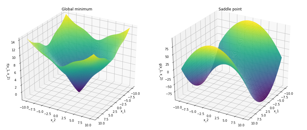
/assets/multidimensional-space-intuition/saddle.png — Figure 1. Examples of a (global) minimum (left), and a saddle point (right).

The saddle points provide a “getaway” direction to the optimizer. While not existent given one dimension, chances that any given critical point is a saddle should increase given more dimensions. To illustrate this, let’s consider the so-called Hessian matrix, which is a matrix of second derivatives of f with respect to all of its arguments.

$\mathbf{H}: h_{i,j} \left[\frac{\partial^2f}{\partial x_i \partial x_j}\right] \quad i,j \in \{1, 2, \cdots, N\}$

As the Hessian is a symmetric matrix, we can diagonalize it.

$\left[\frac{\partial^2 f}{\partial x_i \partial x_j}\right] \xrightarrow{\text{diagonal}} \left[\frac{\partial^2 f}{\partial^2 x_i'}\right] \quad i \in \{1, 2, \cdots, N\}$

The condition for the critical point to be a minimum is that the Hessian matrix is positive definite, which means h₁, h₂, …, hₙ > 0.

Assuming that f, being a complicated function, is not biased towards any positive or negative values, we can assume that changes that for any critical point, P(hᵢ) > 0, as well as P(hᵢ) < 0, is 1/2. Furthermore, if we assume that hᵢ does not depend on any other hⱼ, we can treat P(hᵢ) as independent events, in which case:

$p\left(\bigcap_{i=1}^N h_i > 0\right) = \prod_{i=1}^N p(h_i > 0) = \frac{1}{2^N}$

Similarly, for the maxima:

$p\left(\bigcap_{i = 1}^N h_i < 0\right) = \frac{1}{2^N}$

Chances that our critical point is a saddle point is the chance that it is neither a maximum nor a minimum. Consequently, we can see that:

$\lim_{N\to\infty} p_S = \lim_{N\to\infty} \left(1 - \frac{1}{2^N} - \frac{1}{2^N}\right) = 1$

The high-dimensional space seems, therefore, to be the space of possibilities. The higher the number of dimensions, the more likely it feels that thanks to the saddle points, there will be directions for the optimizer to do its job.

Of course, as we can find examples of functions that would not conform to this statement, the statement is not proof. However, if the function f possesses some complicated dependency on its arguments, we could at least expect that the higher the number of dimensions, the more “forgiving” space would be (on average).

A hyper-ball

A circle, a ball or a hyper-ball - a mathematical description of any of these objects is simple.

$\mathcal{S} = \{x \in \mathbb{R}^{N + 1}: \|x\| \leq r\}$

All that this equation describes is simply a set of points, whose distance from the origin is less or equal to a constant number (regardless of the number of dimensions). It can be shown that for any number of dimensions, the total volume (or hyper-volume) of this object can be calculated using the following formulae:

$V_1(r) = 2r^1 \\ V_2(r) = \pi r^2 \\ V_3(r) = \frac{4}{3}\pi r^3 \\ \vdots \\ V_n(r)=\frac{\pi^{\frac{n}{2}}}{\Gamma(\frac{n}{2}+1)}r^n$

Looking on how it scales with n, we can see that:

$V_n(r) = K_n r^n$

An interesting thing happens if we try to plot this equation for a unit hyper-ball (r = 1), for an arbitrary number of dimensions:

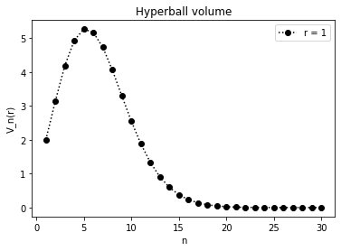
/assets/multidimensional-space-intuition/volume.png — Figure 2. Volume for a hyper-ball of unit radius.

As we can see, for the first few n’s, the volume of the sphere increases. However, as soon as n > 5, it quickly drops to a very small number. Can it be true that the unit hyper-ball is losing mass? To see where the mass goes, let’s define a density parameter:

$\rho(\varepsilon)=\frac{V_n(r)-V_n(r-\varepsilon)}{V_n(r)}$

where epsilon is used to define a “shell” of arbitrary thickness. Again, setting r to 1, and sweeping epsilon from zero to one, we can make an interesting observation:

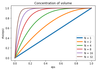
/assets/multidimensional-space-intuition/density.png — Figure 3. Concentration of volume of an N-dimensional ball.

As the number of dimensions grows, it turns out that almost all of the mass of the ball is concentrated around its border.

This property of the high-dimensional space is especially important if we consider drawing samples from some neighborhood that belongs to that space. In silico and Mark Khoury provide interesting illustrations, trying to show what happens when N becomes high. It feels almost as if the dimensionality of space deflects that space, making the confined points wanting to escape or push towards the ends as if they tried to explore the additional degrees of freedom that are available.

A multi-dimensional cake

Let’s consider a cubical cake that we would like to slice N times to create some pieces. If our cake is a three-dimensional cube (we will use K to describe dimensions now), the maximal number of pieces we can divide it to is described by the following sequence:

$c_n^{(3)}=\frac{1}{6}\left(n^3+5n+6\right)={\binom{n}3}+{\binom{n}2}+{\binom{n}1}+{\binom{n}0}$

where

${\binom{n}k}=\frac{n!}{k!(n-k)!}$

is a binomial coefficient.

As before, we can extend our mathematics to more dimensions.

Having a multi-dimensional cake of K dimensions and a multi-dimensional knife to slice is using (K-1)-dimensional hyper-planes, the number of “hyper-pieces” is to be calculated using:

$C_n^{(K)}=\sum_{k=0}^K{\binom{n}k}=\sum_{k=0}^K\prod_{i=1}^k\frac{n+1-i}{i}$

where the latter formula is completely equivalent, but just easier to compute.

Now, let’s see how hyper-pieces count will scale with N and K.

1
2
3
4
5
6
7
8
9
10
11
12
13
14
15
16
17
18
19
20
21
22
23
24
import numpy as np
import pandas as pd
form itertools import product


def cake(n, K):
    c = 0
    for k in range(K + 1):
        term = [(n + 1 - i) / i for i in range(1, k + 1)]
        c += np.array(term).prod()
    return c


N = 10  # cuts
K = 10  # dimensions

p = list(product(range(1, N + 1), range(1, K + 1)))
X = pd.DataFrame(pd.DataFrame((p,)).to_numpy().reshape(N, K)
X.index = range(1, N + 1)
X.columns = range(1, K + 1)
C = X.applymap(lambda x: cake(x[0], x[1])).astype(int)
ns = X.applymap(lambda x: x[0])
ks = X.applymap(lambda x: x[1])
C_normed = C / (nx * ks)

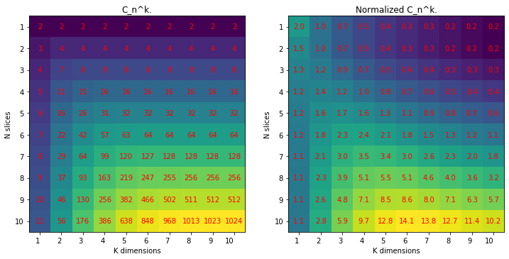
/assets/multidimensional-space-intuition/cake.png — Figure 4. The _N_, _K_ - cake number (left): showing the maximum number of slices of an _K_-dimensional space using _N_ cuts. The normalized cake number _C / (N * K)_, shows how the number of slices scale with when adding dimensions or cuts.

Looking at the left figure, we see the direct result of the above formula. Despite it looks close to exponential, it is still a polynomial expression. Intuitively, the more dimensions or the more cuts, the more pieces we can yield from the cake.

However, if we normalize C by dividing it by the product of N * K, we can see that for some fixed number of cuts, the increase of the number of slices with N does not happen so fast anymore. In other words, it seems that the potential of the space to be divisible to more unique regions is somehow saturated and that for any amount of cuts K, there exists an “optimal” dimension number N, for which space “prefers” to be divided.

Considering that, for example, for a dense neural network layer the output sate y is obtained by the following vector-matrix multiplication:

$\mathbf{y}=g(\mathbf{W}\cdot\mathbf{x})$

where g is an activation function, and

$y_i=\sum_{j}w_{ij}x_j=[w_{i,j-1},...,w_{i,1},w_{i,0}]\cdot[x_{j-1},...,x_1,x_0]^T$

both N and K can be manipulated. As we have seen before, both increasing K (aka the number of features of x) or N (aka the number of hyper-planes) leads to the definition of more regions that can contribute to the unique “firing” patterns of y’s, which are associated with these pieces. The more pieces we ave, the better performance we should expect, but at the same time increasing N and K also means more operations and larger memory footprint. Therefore, if for a given N, the number of slices per every extra dimension added no longer grows, it may be favorable in terms of resource consumption to keep the dense layers smaller?

Conclusions

In this article, we have looked into three aspects of the multidimensionality of space. As we couldn’t visualize it (we didn’t even try…), we took advantage of some mathematical mechanisms to gain a bit more insight into the strange behavior of this world. Although not backed with any ultimate proofs, we hope that the mathematical reasoning just presented can spark some inspiration, intuition, and imagination, which is something that is often needed when having to cope with N-dimensions.

If you have your ideas or opinions (or you would like to point some inconsistency), please share them in the comments below.