Training on batch: how do you split the data?

Introduction

With increasing volumes of the data, a common approach to train machine-learning models is to apply the so-called training on batch. This approach involves splitting a dataset into a series of smaller data chunks that are handed to the model one at a time.

In this post, we will present three ideas to split the dataset for batches:

• creating a “big” tensor,
• loading partial data with HDF5,
• python generators.

For illustration purposes, we will pretend that the model is a sound-based detector, but the analysis presented in this post is generic. Despite the example is framed as a particular case, the steps discussed here are essentially splitting, preprocessing and iterating over the data. It conforms to a common procedure. Regardless of the data comes in for of image files, table derived from a SQL query or an HTTP response, it is the procedure that is our main concern.

Specifically, we will compare our methods by looking into the following aspects:

• code quality,
• memory footprint,
• time efficiency.

What is a batch?

Formally, a batch is understood as an input-output pair (X[i], y[i]), being a subset of the data. Since our model is a sound-based detector, it expects a processed audio sequence as input and returns the probability of occurrence of a certain event. Naturally, in our case, the batch is consisted of:

• X[t] - a matrix representing processed audio track sampled within a time-window, and
• y[t] - a binary label denoting the presence of the event,

where t to denote the time-window (figure 1.).

✕

Figure 1.

An example of data input. Top: simple binary label (random), middle: raw audio channel (mono), bottom: spectrogram represented as naural logarithm of the spectrum. The vertical lines represent slicing of the sequence into batches of 1 second length.

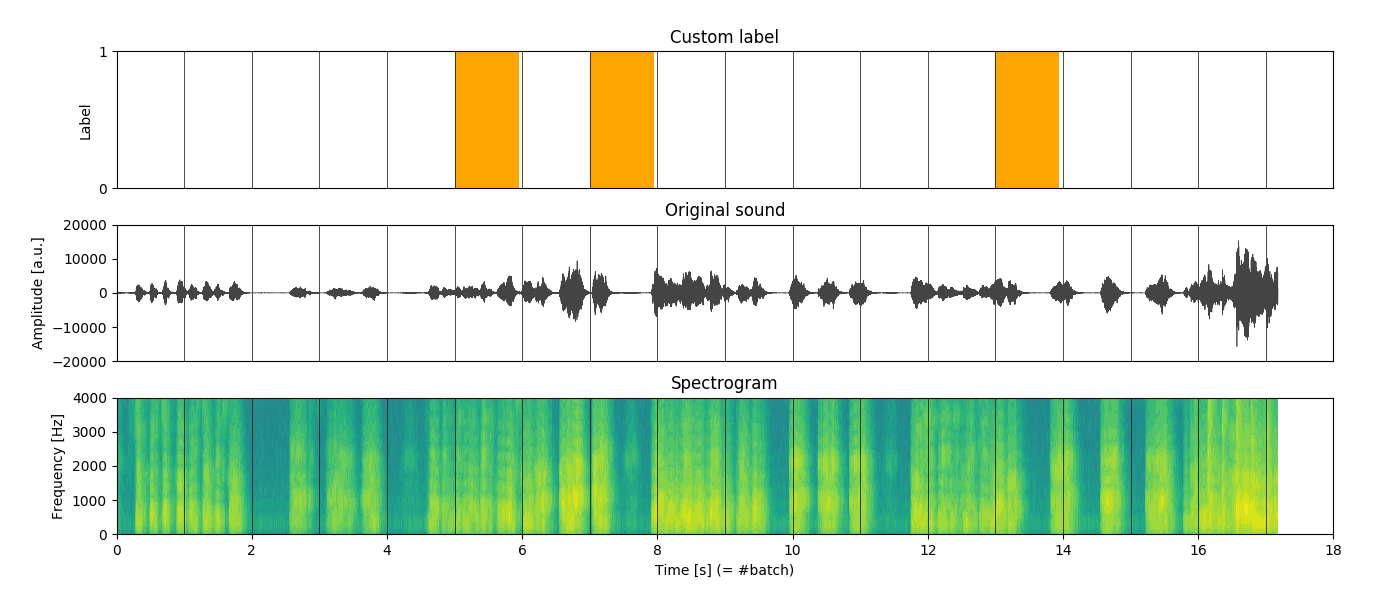
Spectrogram

As for the spectrogram, you can think of it as a way of describing how much of each “tune” is present within the audio track. For instance, when a bass guitar is being played, the spectrogram would reveal high intensity more concentrated on the lower side of the spectrum. Conversely, with a soprano singer we would observe the opposite. With this kind of “encoding”, a spectrogram naturally represents useful features for the model.

Comparing ideas

As a common prerequisite for our comparison, let’s briefly define the following imports and constants.

1
2
3
4
5
6
7
8
9
10
11
12
13
14
15
16
17
from scipy.signal import spectrogram
from os.path import join
from math import ceil
import numpy as np


FILENAME = 'test'
FILEPATH = 'data'
CHANNEL  = 0        # mono track only
SAMPLING = 8000     # sampling rate (audio at 8k samples per s)
NFREQS   = 512      # 512 frequencies for the spectrogram
NTIMES   = 400      # 400 time-points for the spectrogram
SLEN     = 1        # 1 second of audio for a batch

N = lambda x: (x - x.mean())/x.std() # normalization

filename = join(FILEPATH, FILENAME)

Here, the numbers are somewhat arbitrary. We decide to go for the lowest sampling rate (other common values are 16k and 22.4k fps), and let every X-chunk be a spectrogram of 512 frequency channels that is calculated from a non-overlapping audio sequence of 1s, using 400 data points along the time axis. In other words, each batch will be a pair of a 512-by-400 matrix, supplemented with a binary label.

Idea #1 - A “big” tensor

The input to the model is a 2-dimensional tensor. As the last step involves iterating over the batches, it makes sense to increase the rank of the tensor and reserve the third dimension for the batch count. Consequently, the whole process can be outlined as follows:

1. Load the x-data.
2. Load the y-label.
3. Slice X and y into batches.
4. Extract features on each batch (here: the spectrogram).
5. Collate X[t] and y[t] together.

Why wouldn’t that be a good idea? Let’s see an example of the implementation.

1
2
3
4
5
6
7
8
9
10
11
12
13
14
15
16
17
18
19
20
21
22
23
24
25
26
27
def create_X_tensor(audio, fs, slen=SLEN, bsize=(NFREQS, NTIMES)):
    X = np.zeros((n_batches, bsize[0], bsize[1]))

    for bn in range(n_batches):
        aslice = slice(bn*slen*fs, (bn + 1)*slen*fs)
        *_, spec = spectrogram(
                N(audio(aslice)), 
                fs       = fs, 
                nperseg  = int(fs/bsize[1]),
                noverlap = 0,
                nfft     = bsize[0])
        X[bn, :, :spec.shape[1]] = spec
    return np.log(X + 1e-6) # to avoid -Inf

def get_batch(X, y, bn):
    return X[bn, :, :], y[bn]


if __name__ == '__main__':
    audio = np.load(filename + '.npy')[:, CHANNEL]
    label = np.load(filename + '-lbl.npy')

    X = create_X_tensor(audio, SAMPLING)
    for t in range(X.shape[0]):
        batch = get_batch(X, y, t)
        print ('Batch #{}, shape={}, label={}'.format(
            t, X.shape, y[i]))

The essence of this method can best be described as load it all now, worry about it later.

While creating X a self-contained data piece can be viewed as an advantage, this approach has disadvantages:

1. We lead all data into the RAM, regardless of the RAM can store such data or not.
2. We use the first dimension of X for the batch count. However, this is solely based on a convention. What if the next time somebody decides that it should be the last one instead?
3. Although X.shape[0] tells us exactly how many batches we have, we still have to create an auxiliary variable t to help us keep track of the batches. This design enforces the model training code to adhere to this decision.
4. Finally, it asks for the get_batch function to be defined. Its only purpose is to select a subset of X and y and collate them together. It looks undesired at best.

Idea #2 - Loading batches with HDF5

Let’s start with eliminating the most dreaded problem that is having to load all data into the RAM. If the data comes from a file, it would make sense to be able to only load portions of it and operate on these portions.

Using skiprows and nrows arguments from Pandas’ read_csv it is possible to load fragments of a .csv file. However, with the CSV format being rather impractical for storing sound data, Hierarchical Data Format (HDF5) is a better choice. The format allows us to store multiple numpy-like arrays and access them in a numpy-like way.

Here, we assume that the file contains intrinsic datasets called 'audio' and 'label'. Check out Python h5py library for more information.

1
2
3
4
5
6
7
8
9
10
11
12
13
14
15
16
17
18
19
20
21
22
23
24
25
26
27
28
29
def get_batch(filepath, t, slen=SLEN, bsize=(NFREQS, NTIMES)):
    with h5.File(filepath + '.h5', 'r') as f:
        fs    = f['audio'].attrs['sampling_rate']
        audio = f['audio'][t*slen*fs:(t + 1)*slen*fs, CHANNEL]
        label = f['label'][t]

    *_, spec = spectrogram(
            N(audio),
            fs          = fs,
            nperseg     = int(fs/bsize[1]),
            noverlap    = 0,
            nfft        = bsize[0])
    X = np.zeros((bsize[0] // 2 + 1, bsize[1]))
    X[:, :spec.shape[1]] = spec
    return np.log(X + 1e-6), label

def get_number_of_batches(filepath):
    with h5.File(filepath + '.h5', 'r') as f:
        fs = f['audio'].attrs['sampling_rate']
        sp = f['audio'].shape[0]
    return ceil(sp/fs)
    

if __name__ == '__main__':
    n_batches = get_number_of_batches(filename)
    for t in range(n_batches):
        batch = get_batch(filename, t)
        print ('Batch #{}, shape={}, label={}'.format(
            i, batch[0].shape, batch[1]))

Hopefully, our data is now manageable (if it was not before)! Moreover, we have also achieved some progress when it comes to the overall quality:

1. We got rid of the previous get_batch function and replaced it with the one that more meaningful. It computes what is necessary and delivers the data. Simple.
2. Our X tensor no longer needs to be artificially modified.
3. In fact, by changing get_batch(X, y, t) to get_batch(filename, t), we have abstracted access to our dataset and removed X and y from the namespace.
4. The dataset has also became a single file. We do not need to source the data and the labels from two different files.
5. We do not need to supply fs (the sampling rate) argument. Thanks to the so-called attributes in HDF5, it can be a part of the dataset file.

Despite the advantages, we are still left with two… inconveniences.

Because the new get_batch does not remember the state. We have to rely on controlling t using a loop as before. However, as there is no mechanism within get_batch to tell how large the loop needs to be (apart from adding the third output argument, making it weird), we need to check the size of our data beforehand. Apart from adding the third output to get_batch, which would make this function rather weird, it requires us to create a second function: get_number_of_batches.

Unfortunately, it does not make the solution as elegant as it can be. If we only transform get_batch to a form where it would preserve the state, we can do better.

Idea #3 - Generators

Let’s recognize the pattern. We are only interested in accessing, processing and delivering of data pieces one after the other. We do not need it all at once.

For these opportunities, Python has a special construct, namely generators. Generators are functions that return generator iterators Instead of eagerly performing the computation, the iterators deliver a bit of the result at the time and wait to be asked to continue. Perfect, right?

Generator iterators can be constructed in three ways:

• through an expression that is similar to a list comprehansion: e.g. (i for i in iterable), but using () instead of [],
• from a generator function - by replacing return with yield, or
• from a class object that defines custom __iter__ (or __getitem__) and __next__ methods (see docs).

Here, using yield fits naturally in what we need to do.

1
2
3
4
5
6
7
8
9
10
11
12
13
14
15
16
17
18
19
20
21
22
def get_batches(filepath, slen=SLEN, bsize=(NFREQS, NTIMES)):
    with h5.File(filepath + '.h5', 'r') as f:
        fs = f['audio'].attrs['sampling_rate']
        n_batches = ceil(f['audio'].shape[0]/fs)

        for t in range(n_batches):
            audio = f['audio'][t*slen*fs:(t + 1)*slen*fs, CHANNEL]
            label = f['label'][t]
            *_, spec = spectrogram(
                    N(audio),
                    fs          = fs,
                    nperseg     = int(fs/bsize[1]),
                    noverlap    = 0,
                    nfft        = bsize[0])
            X = np.zeros((bsize[0] // 2 + 1, bsize[1]))
            X[:, :spec.shape[1]] = spec
            yield np.log(X + 1e-6), label


if __name__ == '__main__':
    for b in get_batches(filename):
        print ('shape={}, label={}'.format(b[0].shape, b[1]))

The loop is now inside of the function. Thanks to the yield statement, the (X[t], y[t]) pair will only be returned after get_batches be called t - 1 times. The model training code does not need to manage the state of the loop. The function remembers its state between calls, allowing the user to iterate over batches as opposed to having some artificial batch index.

It is useful to compare generator iterators to containers with data. As batches get removed with every iteration, at some point the container becomes empty. Consequently, neither indexing nor a stop condition is necessary. Data gets consumed until there is no more data and the process stops.

Performance: time and memory

We have intentionally started with a discussion on the code quality, as it was tightly related to the way our solution has been evolving. However, it is just as important to consider resource constraints, especially when data grows in volume.

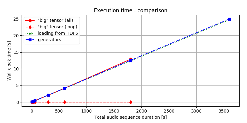
Figure 2. presents the time it takes to deliver the batches using the three different methods described earlier. As we can see, the time it takes to process and hand over the data is nearly the same. Regardless if we load all data to process and then slice it or load and process it bit-by-bit from the beginning, the total time to get the solution is almost equal. This, of course, could be the consequence of having SSD that allows faster access to the data. Still, the strategy chosen seems to have little impact on overall time performance.

✕

Figure 2.

Time performance comparison. The red-solid line refers to timing both loading the data to the memory and performing the computation. The red-dotted line times only the loop, where slices are delivered, assuming that data was precomputed. The green-dotted line refers to loading batches from HDF5 file and the blue-dashed-dotted line implements a generator. Comparing the red lines, we can see that just accessing of the data once it is in the RAM is almost for free. When data is local, the differences between the other cases are minimal, anyway.

Much more difference can be observed when looking at figure 3. Considering the first approach, it is the most memory-hungry of all, making the 1-hour long audio sample throws MemoryError. Conversely, when loading data in chunks, the allocated RAM is determined by the batch size, leaving us safely below the limit.

✕

Figure 3.

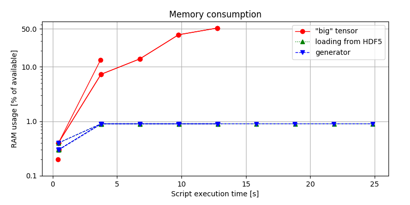
Memory consumption comparison, expressed in terms of the percentage of the available RAM being consumed by the python script, evaluated using: (env)$ python idea.py & top -b -n 10 > capture.log; cat capture.log | egrep python > analysis.log, and post-processed.

Surprisingly (or not), there is no significant difference between the second and the third approach. What the figure tells us, is that choosing or not choosing to implement a generator iterator makes no impact on the memory footprint on our solution.

This is an important take-away. It is often encouraged to use generators as more efficient solutions to save both time and memory Instead, the figure shows that generators alone do not contribute to better solutions in terms of the resources. What matters is only how quickly we can access the resources and how much data we can handle at once.

Using an HDF5 file proves to be efficient since we can access the data very quickly, and flexible enough that we do not need to load it all at once. At the same time, the implementation of a generator improves code readability and quality. Although we could also frame the first approach in a generator form, it would not make any sense, since, without the ability to load data in smaller quantities, generators would only improve the syntax. Consequently, the best approach seems to be the simultaneous usage of loading partial data and a generator, which is represented by the 3rd approach.

Final remarks

In this post, we have presented three different ways to split and process our data in batches. We compared both the performance of each of the approaches and the overall code quality. We have also stated that the generators on their own do not make the code more efficient. The final performance is dictated by the time and memory constraints, however, generators can make the solution more elegant.

What solution do you find the most appealing?