Categorical sequences with Pandas for household expense control

Introduction

Dealing with household expenses is never pleasant. Although banks try to make it fun these days, it is seldom that their user interface would actually help you to gain insight into how much you actually spend and on what “it all goes”. After all, the more you spend, the more likely you are to apply for a loan, correct?

Anyways, most banks offer their customers an option to download of a transaction history. While the options usually include CSV formatting, the lists are all but easy for the actual analytics.

In this post, we show how to translate such historical data into an easier to analyse format using pandas library - one of the “must-knowns” for any data scientist.

Initial format

The initial format is typical for historical data. It contains a date or a time-stamp, a transferee and an amount that was transferred:

1
2
3
4
5
6
      DATE                 RECIPIENT   VALUE   ACCOUNT       CATEGORY
2019-04-06     Popular Kiosk Network  -14.30  personal           Food
2019-04-06     Pharmacy at Warsaw st.  -9.86  personal        Hygiene
2019-04-06       American Cinema Ltd. -61.06    shared  Entertainment
2019-04-06  Unhealthy Food Chain Ltd. -31.10    shared           Food
2019-04-06              Fancy Donuts  -12.34    shared           Food

It is definitely not analytics-friendly, and we would like to present the values on a timeline with different categories. For that, we will formulate a table, where each column’s name matches the value taken from the CATEGORY column. Then we will accummulate the data within time-periods in order to make it easy to track the expenses within each category against time.

Processing

To categories

As the first step, we need to access the data, which can either be done by namually downloading the file or requesting the data through a bank open API (if available).

1
2
3
4
import pandas as pd

xl = pd.ExcelFile(FILEPATH)
df = xl.parse()

Once we have the initial table loaded as Pandas DateFrame, we can pick the new columns’ names from the values of CATEGORY.

1
2
3
4
5
6
7
8
9
10
11
df['CATEGORY'] = df['CATEGORY'].fillna('Other')
new_columns = df['CATEGORY'].unique()
categories = [0]*len(new_columns)

cnt = 0
for dim in new_columns:
    categories[cnt] = df[df['CATEGORY'].str.match(dim)].loc[:, df.columns != 'CATEGORY']
    categories[cnt] = categories[cnt][['DATE', 'VALUE']]
    categories[cnt] = categories[cnt].rename(columns={'VALUE': dim.upper()})
    cnt += 1
df2 = pd.concat(categories).sort_values('DATE')

The first line replaces all empty values (appearing as NaNs) with common category “Other”. The second line uses the CATEGORY values to create a list of new column names.

In the loop, we use df[df['CATEGORY'].str.match(dim)] construction to pick all the actual values that belong to the given category. At the same time, the .loc[:, df.columns != 'CATEGORY'] removes the whole column as it is now completely redundant. Finally, we limit the sub-table to contain only the DATE and VALUE columns, from where we replace the name "VALUE", with the one matching our category (dim). At last, we concatenate all the sub-tables and sort them with respect to the time stamp.

Our data is now of the following form:

1
2
3
4
5
6
7
         DATE  ENTERTAINMENT    FOOD   HYGIENE  ...
0  2019-04-06         -14.30     NaN       NaN  ...
1  2019-04-06            NaN   -9.86       NaN  ...
2  2019-04-06            NaN     NaN    -61.06  ...
3  2019-04-06            NaN  -31.10       NaN  ...
4  2019-04-06            NaN  -12.34       NaN  ...
          ...            ...     ...       ...  ...

To sequences

So far so good. We have one table now that contains all values on “per category” basis. Unfortunately, it does contain a lot of “holes” (NaNs), which still hinder the nice overview. Furthermore, in this example we only have Dates, so our time-resolution is equal to one day, although we may have several entrances within one day. In many situations, we may have data that is time-stamped all the way to miliseconds, and there would actually be no point in keeping such high resolution.

Let’s say we are only interested in our weekly spending within each of the categories listed. Pandas offers a lot of tools for handling of the sequential data.

1
2
3
ts = pd.to_datetime(df2['DATE'])
df2 = df2.set_index(ts)
df3 = df2.resample('7D').sum()

Here, we use pd.to_datefime() to batch-convert our timestamps from strings to date-time objects. Once done, we change it to be our actual index. Finally, given that our index is now a date-time object, we can resample it to form 7-days time bins, and sum all the expenses within these bins.

Our data is not in the following form:

1
2
3
4
5
6
7
8
            ENTERTAINMENT     FOOD  HYGIENE  ...
DATE                                       
2019-03-05            0.0     0.00     0.00  ...
2019-03-12            0.0     0.00   -79.33  ...
2019-03-19          -13.0 -1035.15   -28.66  ...
2019-03-26          -24.0 -1421.84  -215.30  ...
2019-04-02         -187.4  -347.93  -221.43  ...
       ...            ...     ...       ...  ...

This operation applies automatically to all the columns we have, at the same time treating all NaNs as zeros. As a result, we obtain a multi-dimensional time-continues table, which contains our weekly spendings on things grouped by the joint category.

Now, let’s use the derived table to plot the data.

1
2
3
4
5
6
7
8
9
10
11
12
13
14
15
16
17
%pylab

fig, ax = plt.subplots()

df4   = df4.reset_index()
cols  = [c for c in df4.columns if c in ['Entertainment', 'Food', 'Hygiene', 'House']]
tline = df4['Date'].dt.strftime('%Y-%m-%d')

ax.bar(tline, -1*df4.sum(axis=1), color='k')
ax.plot(tline, -1*df4[cols], "o-")
ax.tick_params(axis='x', rotation=45)
ax.set_xlabel('Time')
ax.set_ylable('Expences [gold pcs.]')

plt.title('Example')
plt.legend(cols + ['Balance'])
plt.show()

As a result, we get the following plot.

✕

Figure 1.

Example of the analytics.

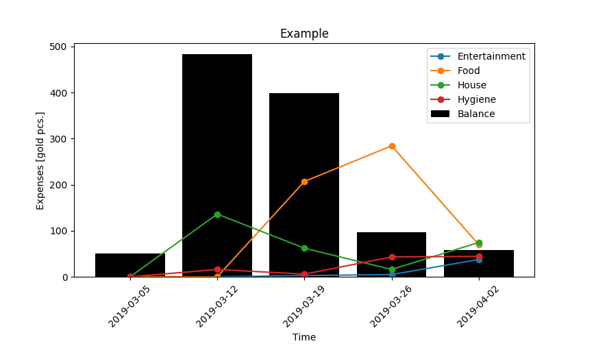
Isn’t that nice?