
Decision Tree - Implemented from scratch
Introduction
It is not hard to be under an impression that the world is all about neural networks these days when it comes to making models. Many teams seem to brag about super-cool architectures as if getting enough quality data was straightforward, GPU racks were open 24/7 (for free), and their customer’s patience was set to infinity.
In this article, we will present one of the most basic machine-learning algorithms known as a Decision Tree. Decision trees are often recognized as “rescue” models, as they do not require large quantities of data to work and are easy to train. Despite being prone to overfitting, the trees have a great advantage of being explainable due to the nature of their prediction mechanism.
Traditionally, we will implement and train the model from scratch, with bare-bone numpy and pandas. Note that our way of implementing it is, by all means, not the only one possible. Here, we focus on explaining the inner working of the algorithm by designing our tree from the first principles. Therefore, take it more as a demo rather than a production solution that you can find e.g. in scikit-learn.
Theory
Decision tree owes its names due to its structure that resembles a tree. A tree that is trained will pass an example data through a sequence of nodes (also called “splits”, but more of that later). Every node serves as a decision point for to what is to be the next node. The final node, a “leaf”, is equivalent to a final prediction.
The training process
Training a decision tree is a process of identifying the most optimal structure of nodes. To explain this, consider an -dimensional input feature vector for whom we want to identify a target class. The first node needs to “know” which of the vector’s components to check and what would be the threshold value to check against. Depending on the decision, the vector will then be routed to a different node, and so on.
A well-trained tree would have its nodes, and their respective parameters chosen in such a way, that the number of wrongly recognized target classes is the lowest. Now, the question is how do construct such nodes?
Here, there are at least two mathematical formulae that can help us out.
Cross-entropy formula
Gini coefficient (gini impurity)
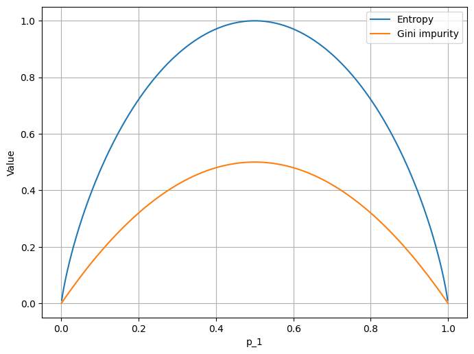
Both of these formulae express some sort of information about the system. As the cross-entropy function looks very similar to the gini impurity (figure 1.), we can use any of them to build our intuition (and the model). However, for clarity, let’s use the latter.
Interpretation
As mentioned earlier, both of the functions express some sort of information. Consider a binary classification system (in which case the number of classes is , and we can only bet if a given example should be assigned a given label or not). From the classification point of view, the safest situation takes place if can know what the outcome should be. In this case, the probability associated with the outcome would either be zero or one. Since for , , the gini impurity in such case is zero. The system is “pure”, in a sense we know what to expect.
Now, as soon as we are not sure (), , reaching its peak exactly when we know the least . The same happens with entropy. The higher it is, the more “chaotic” the system is or we have the least of the “information”.
Adding more classes does not change the logic here. Both figures take the contribution from all the classes through the sum .
Reducing the impurity
OK, but how does the gini impurity help us solve the problem of training a decision tree? As stated earlier, it is all about setting the nodes strategically, so they all contribute to making good decisions. Any decision (any node) is equivalent to slicing or splitting the parameter space along a given axis at some particular value . A “good” decision is more likely to be made if are chosen the way that our knowledge about the system progressively increases. In other words, there are less uncertainty in the two nearly formed subspaces than there was in the beginning.
If and are the gini impurity values associated with the subspaces after the split, we can define the so-called gini gain to be:
where is the example count, and and refer to the subspaces.
The higher the gain , the “wiser” node will be at discriminating different cases. If all nodes are chosen that way, we may have a reasonable model.
Implementation
Let’s create a simple artificial dataset, where every example is represented as a three-dimensional vector .
1
2
3
4
5
6
7
8
9
10
11
12
13
14
15
16
17
import numpy as np
import pandas as pd

from sklearn.datasets import make_classification

X, y = make_classification(
        n_samples=12,
        n_classes=3,
        n_clusters_per_class=2,
        n_features=3,
        n_informative=3,
        n_redundant=0,
        n_repeated=0,
        random_state=42)

df = pd.DataFrame(X, columns=[x for x in range(X.shape[1])])
df["target"] = y
Here, we use pandas only for convenience “to keep things together”. The most important thing is that we have three-dimensional data () as well as three target classes (). The table below presents the dataset.
| 0 | 1 | 2 | target |
|---|---|---|---|
| 0.78 | -1.09 | -0.99 | 0 |
| 1.56 | 0.87 | -0.93 | 1 |
| 1.17 | -0.25 | 0.54 | 0 |
| -1.84 | -0.70 | -2.71 | 2 |
| -1.91 | -1.57 | 0.98 | 1 |
| -0.96 | -0.77 | -3.92 | 2 |
| -0.83 | -2.70 | -2.13 | 0 |
| 0.02 | 2.20 | -0.08 | 2 |
| 1.62 | 0.38 | 0.83 | 0 |
| -0.14 | -0.70 | 1.39 | 1 |
| 2.29 | 0.48 | 0.32 | 1 |
| 0.53 | 2.33 | -0.12 | 2 |
Gini impurity
Calculating the gini coefficient is something we will be doing again and again. Therefore, it makes sense to wrap it as a function.
1
2
3
4
5
def gini(df):
    probs = {}
    for c in df["target"].unique():
        probs[c] = len(df.query("target == @c")) / len(df)
    return sum([p * (1 - p) for p in probs.values()])
The whole function is an implementation of the previously stated formula for .
We iterate over the target classes (line 3.), and obtain the probabilities
by counting events.
Gini gain
Having the code for the gini impurity, let’s create a function for gini gain.
1
2
3
4
5
6
7
8
9
10
11
def gini_gain(df, feature_name, feature_value):
    df_a = df.query(f"{feature_name} < @feature_value")
    df_b = df.query(f"{feature_name} >= @feature_value")

    total_gini = gini(df)
    gini_a = gini(df_a)
    gini_b = gini(df_b)

    m, m_a, m_b = len(df), len(df_a), len(df_b)

    return total_gini - gini_a * m_a / m - gini_b * m_b / m
Naturally, the value of gain depends on the particular choice of (feature_name)
and (feature_value).
Therefore, the function must take them as inputs.
Then, we simply split the dataset into two parts with ( and replaced with _a
and _b) and return the value of the gain.
Finding the best split
Functions gini and gini_gain are only tools.
To find the best split , we need to compare various options
and choose the one that maximizes the gain.
The simplest way to do it is to iterate over the existing dimensions (
and sweep the threshold along that dimension,
each time evaluating the gain.
1
2
3
4
5
6
7
8
9
10
11
12
13
14
15
16
17
18
19
20
21
22
23
24
def find_best_split(df, density_per_feature=10):
    splits = pd.DataFrame()

    for feat in [feat for feat in df.columns if feat != "target"]:
        split_candidates = np.linspace(
            df[feat].min(),
            df[feat].max(),
            num=density_per_feature,
        )

        _splits = pd.DataFrame()
        _splits["candidate_values"] = split_candidates
        _splits["feature"] = feat
        _splits["gini_gain"] = _splits["candidate_values"].apply(
            lambda value: gini_gain(df, feat, value)
        )

        splits = pd.concat([splits, _splits])

    best_split = splits.sort_values(by="gini_gain", ascending=False) \
        .iloc[0]

    return best_split["feature"].iloc[0], \
           best_split["candidate_values"].iloc[0]
As you can see, density_per_feature is an additional argument to choose
the granularity of our sweep (generally the larger the better, but also longer).
The loop in line 4. is the loop over .
Then, we define split and _split purely for convenience.
Having these auxiliary dataframes, we may use the .apply method
to automatically get the gini gain figure for every entry of the frame
and use .sort_values to find the best option.
Once identified, we return both the dimension of choice for the node
as well as the value for the threshold.
The tree
The decision tree is composed of nodes.
When training, we not only need to make the nodes “optimal” but also we need to create
the whole tree structure, so the nodes work together.
While for the nodes we have the find_best_split function, we need to organize them as a tree.
To understand the recursion, one has to first understand the recursion.
Consider the following function:
1
2
3
4
5
6
7
def func(tree, max_iter=5):
    max_iter -= 1
    if max iter <= 0:
        return [max_iter]
    node = [max_iter, func(tree, max_iter)]
    tree.append(node)
    return node
This is a recursive function. It subsequently builds a simple tree (or a “twig” rather…), by nesting the consecutive numbers just like this:
1
2
3
4
tree = func([])
print(tree)

[4, [3, [2, [1, [0]]]]]
As you can see, the process of calling func continues until it hits the max_iter condition.
Until then, it keeps invoking itself and adding nodes to the structure.
Our decision tree is a binary tree (every node branches out to two sub-nodes).
Therefore, we need to modify func a bit to support mode sub-nodes
and replace a single number with a pair .
Consequently, we can accept a convention, where every node is defined by a list of four elements:
- splitting feature (or dimension) ,
- splitting value (the threshold) ,
- sub-node that responds if the decision condition is true,
- sub-node that responds if the decision condition is false.
In addition, we need to define a stop condition to prevent the endless recurring chain. We can agree to apply the following:
- Once we are left with all elements of a single class only for a given sub-node, it means have identified a label for a particular sequence of decision nodes. We may therefore store a class label instead.
- If we suspect that the tree may be going too deep, we may also terminate the recursion and take the average (or mode) of the classes. The model will be less precise, but it would train faster.
Growing the tree
Let’s replace the name func with split and rework the inner part.
1
2
3
4
5
6
7
8
9
10
11
12
13
14
15
16
17
18
19
20
21
22
23
24
25
26
27
28
def split(tree, df, max_depth=5):

    splitting_feature, splittng_value = find_best_split(df)

    df_a = df.query(f"{splitting_feature} < @splitting_value")
    df_b = df.query(f"{splitting_feature} >= @splitting_value")

    max_depth -= 1

    if len(df_a) == 0 or len(df_b) == 0 or max_depth == 0:
        target_a = set(df_a["target"]) if len(df_a) > 0 else set([])
        target_b = set(df_b["target"]) if len(df_b) > 0 else set([])
        target = target_a.union(target_b)

        node = [splitting_feature, splitting_value, target, target]
        return node

    node = [
        splitting_feature,
        splitting_value,
        split(tree, df_a, max_depth=max_depth),
        split(tree, df_b, max_depth=max_depth),
    ]
    tree.append(node)
    return node


tree = split([], df, max_depth=10)
Now, we break it down.
If you look carefully, the split function works recursively just like func.
The difference is how we construct each node.
Here, after we identify the best pair for a given node, and
split the dataset into two subsets, we test against whether we have reached our stop condition.
If any of the subsets df_a and df_b lacks elements, it means we have reached a leaf
and there will be no more splits stemming from the node.
At the same time, either target_a or target_b is an empty set and so
the target, which is a union of the sets, will contain the remaining labels.
Unless we terminated the process prematurely (through max_iters) the set operation
will squash the labels into a single-element set.
This way, we not only identify the target class uniquely but also stick with the convention
of having nodes defined as four-element lists, from which the two last elements are iterable,
which prevents a TypeError exception.
If the condition does not apply, the process continues. In this case, each node “remembers” the most optimal parameters as well as the two sub-nodes that stem off the current one.
An example of a trained tree may look like this:
1
2
3
4
5
6
7
8
9
10
11
12
13
14
15
16
[2, 0.208,
    [1, -1.023,
        [0, -0.839, {0}, {0}],
        [0, 0.804,
            [0, -1.845, {2}, {2}],
            [0, 1.5628, {1}, {1}]
        ]
    ],
    [1, -0.429,
        [0, -1.915, {1}, {1}],
        [0, 2.166,
            [0, 1.172, {0}, {0}],
            [0, 2.290, {1}, {1}]
        ]
    ]
]
The tree as a model
Although this nested structure may not look pleasing, it is very simple for a machine to understand. A model based on this tree simply needs to use the first element of the list to pick the feature to check, compare it against the second element, and depending on the result, forward the question to either third or the fourth element. And repeat the process until what it gets is a set, and return its content as a prediction.
Let’s implement such a model.
1
2
3
4
5
6
7
def model(tree, data):
    node = tree
    while not isinstance(node, set):
        feature = node[0]
        value = node[1]
        node = node[2] if data[feature] < value else node[3]
    return list(node)[0]
Now, we can run this model against the dataset using the .apply method:
1
2
3
df["predicted"] = df.get([0, 1, 2]).apply(
    lambda row: model(tree, row.to_numpy()), axis=1
)
Note that the [0, 1, 2] list refers to the features’ names.
The results are presented in the table below.
| 0 | 1 | 2 | target | predicted |
|---|---|---|---|---|
| 0.784972 | -1.09651 | -0.999525 | 0 | 0 |
| 1.56221 | 0.876346 | -0.937159 | 1 | 1 |
| 1.1727 | -0.258296 | 0.542743 | 0 | 0 |
| -1.84585 | -0.703202 | -2.71293 | 2 | 2 |
| -1.91564 | -1.57344 | 0.982937 | 1 | 1 |
| -0.966766 | -0.774834 | -3.92814 | 2 | 2 |
| -0.839739 | -2.70451 | -2.13491 | 0 | 0 |
| 0.0284821 | 2.20555 | -0.0827445 | 2 | 2 |
| 1.62031 | 0.382993 | 0.835343 | 0 | 0 |
| -0.144515 | -0.700331 | 1.39023 | 1 | 1 |
| 2.29084 | 0.486279 | 0.323968 | 1 | 1 |
| 0.532064 | 2.33869 | -0.120604 | 2 | 2 |
Conclusions
As you can see, the decision tree is quite easy but the implementation may be non-trivial. Anyways, in any production code, we would strongly recommend that you use an already existing implementation. Furthermore, you should probably also look into the so-called ensemble methods such as random forest that may give you an additional boost to the accuracy thanks to combining strengths of several models.