Financial Independence - simulating ODEs with python

May 24, 2020

Introduction

Imagine one day you wake up and you know you are free to do whatever you like for the rest of your life… and… money is no longer a problem. You became truly financially independent and you no longer need to work to make it the next year. Does it sound appealing?

While it may sound so, the path towards that goal is certainly not easy (unlike what Youtube Ads say about it). There exist many factors to be taken into consideration when dealing with your finance and reasoning is often obscured by the complexity.

In this article, we are going to attack the problem mathematically and programmatically.

We will model your wallet using a set of ordinary differential equations (ODEs) and we will later solve using scipy library and Python. At each stage, we will try to link the mathematical formulae with python code and explain the reasoning behind it.

The goal will be to make the model explainable and expandable. We will create it step by step and, hopefully, that will reward us with a more intuitive understanding of both underlying math as well as the code. For reference, please take a look at the following notebook: .

Disclaimer

Before we jump into the equations, we would like to stress that this post should, under no circumstances, be treated as financial advice. The author of this post has a background in physics rather than finance, so please also forgive any possible inconsistencies in the vocabulary used.

Problem statement

There are two ways to look at your wallet.

One way is to look at how much money you have $x(t)$ at any given point in time $t$ . Another way is to look at how it changes in time. Knowing the initial amount $x_0 = x(0)$ as well as the first derivative $\frac{dx}{dt}$ , you can predict what the future holds.

Because formulating equations for the derivative is, in our opinion, a much simpler process, we will favor this approach instead of looking for $x(t)$ directly. After all, once we have a complete expression for $\frac{dx}{dt}$ , $x(t)$ can be found by numerically integrating $\frac{dx}{dt}$ :

$x(t) = \int_0^t \frac{dx}{dt} dt,$

provided we know $x_0$ .

Simple model

You work nine-to-five…

Let’s begin with a simple case, where you just have a job. You don’t invest just yet and your yearly balance is determined by the following three factors:

your yearly income – $a(t)$ ,
all your spending… everything: food, rent, car, drinks, whatever – $s(t)$ ,
the tax that you pay on your income – $T(a)$ .

If nothing else comes into play, your gain (or loss) – the rate at which you are getting rich or poor is:

$\Delta = a(t) - s(t) - T(a).$

Therefore, we can set

$\frac{dx}{dt} = \Delta.$

If $a, s$ and $T$ are constants, the equation is, in fact, so simple that we can solve it analytically:

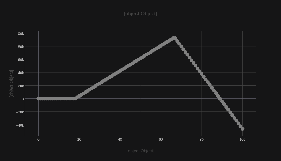
$\int_{x(0)}^{x(t)} dx = \int_0^t \Delta dt \quad \Rightarrow \quad x(t) = \Delta t + x_0.$

It is a straight line, but as we are just setting up the path to gradually add complexity, let’s do it in python.

1
2
3
4
5
6
7
8
9
10
11
12
13
14
15
16
17
18
19
20
21
22
23
import numpy as np
import pandas as pd
from scipy.integrate import odeint


class Life:
    def __init__(self):
        self.income = 10000  # gold pcs. per month
        self.spending = 5000 # gold pcs. per month
        self.tax_rate = 0.19 # example
    
    def earn(self, t):
        return 12 * self.income

    def spend(self, t):
        return 12 * self.spending

    def pay_taxes(self, t):
        return self.earn(t) * self.tax_rate


def live_without_investing(x, t, you):
    return you.earn(t) - you.spend(t) - you.pay_taxes(t)

Here, Life is the class, whose methods we will use to define the fractional contributions. While its form is purely a matter of convenience, it makes sense, to keep the definitions of the contributions separate as they can themselves grow in complexity (e.g. progressive tax).

The live_without_investing(...) function is our derivative, and as such, it has a precisely defined interface func(x, t, **args).

To perform the integration, we can use odeint from scipy.

1
2
3
4
5
6
7
8
def simulate(you):
    t = np.linspace(0, 100, num=101)
    x = odeint(live_without_investing, 0, t, args=(you,))
    return pd.DataFrame({'time': t, 'wallet (non-investor)': x})


you = Life()
df = simulate(you)

Here, we defined a timeline of 100 (years) with a granularity of 1, and passed it as the third argument to odeint. The zero passed as the second argument represents $x_0 = 0$ that is our initial condition. The fourth (optional) argument allows us to pass additional arguments to the function, which we just did by passing you object.

Life’s discontinuities

It’s hard to imagine that you had been paying taxes when you were five. Similarly, past a certain age, you probably would like to reap the harvest of your work.

To incorporate those key changes in your life, we will split it into three stages:

Childhood – where you were entirely dependent on your parents, thus $x(t) = 0$ .
Active life – you earn, you spend, you pay taxes.
Retirement – your income is replaced with a pension that is lower than the income, your spending stays purposely at the same level, but tax is assumed to be already paid.

At the same time, we introduce two more parameters: you.starting_age and you.retirement_age to be the years of your life that you transition between the stages mentioned above.

For our mathematical model, this transitioning implies the existence of two points $t_1$ and $t_2$ , at which $\frac{dx}{dt}$ is discontinuous. To properly compute $x(t)$ , we need to piece-wise integrate $\frac{dx}{dt}$ over your life, from the cradle to the grave.

$x(t) = \int_{\text{birth}}^{t1} \frac{dx}{dt} dt + \int_{t1}^{t2} \frac{dx}{dt} dt + \int_{t2}^{\text{death}} \frac{dx}{dt} dt$

For our code, we modify the model in the following way:

1
2
3
4
5
6
7
8
9
10
11
12
13
14
15
16
17
18
19
20
21
22
23
24
class Life:
    def __init__(self):
        ...  # as before
        self.pension = 1000
        self.starting_age = 18
        self.retirement_age = 67

    def earn(self, t):
        if t < self.starting_age:
            return 0
        elif self.starting_age <= t < self.retirement_age:
            return 12 * self.income
        else:
            return 12 * pension

    def spend(self, t):
        ...  # as before

    def pay_taxes(self, t):
        ...  # as before


def life_without_investing(x, y, you):
    ...  # as before

Then, the simlulation becomes:

1
2
3
4
5
6
7
8
9
10
11
12
13
def simulate(you):
    t0 = np.linespace(0, you.starting_age - 1, num=you.starting_age)
    t1 = np.linespace(you.starting_age, you.retirement_age - 1, num=(you.retirement_age - you.starting_age))
    t2 = np.linespace(you.retirement_age, 100, num=(100 - you.retirement_age))

    x0 = np.zeros((t0.shape[0], 1))
    x1 = odeint(live_without_investing, 0, t1, args=(you,))
    x2 = odeint(live_without_investing, x1[-1], t2, args=(you,))

    df0 = pd.DataFrame({'time': t0, 'wallet (non-investor)': x0})
    df1 = pd.DataFrame({'time': t1, 'wallet (non-investor)': x1})
    df2 = pd.DataFrame({'time': t2, 'wallet (non-investor)': x2})
    return pd.concat([df0, df1, df2])

Note that we also feed $x(t_n)$ as an initial condition to the next integral. Although $\frac{dx}{dt}$ are discontinuous, we cannot say the same about $x(t)$ !

/assets/financial-independence-ode-python/case-1-non-investor.png — Figure 1. Example using `starting_age = 18`, `retirement_age = 67`, income = 1000`, `costs = 650`, `tax_rate = 19%`. Observe that once the retirement age is past, the pension does not compensate with the spending, subsequently leading to debt.

Adding non-linearities

So far, we assumed that the yearly increase to the wallet was a constant function $\Delta = a - s - T(a), \Delta \neq \Delta(t)$ . You would likely receive some yearly salary raise or increase your spending. It is also possible that the tax rate itself you may want to model as a time-dependent function.

Let’s say that your income is now a linear function of time $a(t) = \alpha_0 + \alpha_1 t$ , where $\alpha_0$ is your expected base income (average) and $\alpha_1$ is the amount of extra “gold pcs.” you would receive every year. Similarly, the spending can also take the form of $s(t) = \sigma_0 + \sigma_1 t$ , with $\sigma_0$ being the average monthly spending and $\sigma_1$ is the extra amount you would be spending in the future - a sort of “inflation of the living standard”.

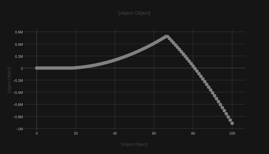
Now, our derivative of $x$ is proportional to time $\frac{dx}{dt} \propto t$ , hence we can expect $x(t)$ to be quadratic $x(t) \propto t^2$ .

Again, programmatically:

1
2
3
4
5
6
7
8
9
10
11
12
13
14
15
16
17
18
class Life:
    def __init__(self):
        ...  # as before
        self.pay_raise = 100
        self.life_inflation = 50

    def earn(self, t):
            ...  # as before
        elif self.starting_age <= t < self.retirement_age:
            return 12 * (self.income + self.pay_raise \
                      * (t - self.starting_age))
        else:
            ...  # as before

    def spend(self, t):
        ...  # as before
        return 12 * (self.costs + self.life_inflation \
                  * (t - self.starting_age))

The integration stays the same, but it brings a new result.

/assets/financial-independence-ode-python/case-2-non-investor.png — Figure 2. Example using additional parameters: `pay_raise = 100`, `life_inflation = 50`. Observe the parabolic shape of both curves.

Investing

If you follow the computations, you may have tried to forecast your financial condition based on numbers more relevant to you. You have probably noticed, that even if you choose not to expand your living standards $\sigma_1 = 0$ , even a high average pay raise $\alpha_1$ does not guarantee an early or safe retirement.

Mathematically, you are free to construct whatever “pay raising” terms you want (e.g. $a(t) \propto t^2$ or $a(t) \propto t^3$ ), but you will probably have a hard time trying to justify their practical origins. Besides, such terms can only give your wallet polynomial growth, which is, to be honest, not as fast as it can get.

At this stage, some of you may already recall the formula for the compound interest:

$\text{FV} = \text{PV}\left(1 + \frac{R}{n}\right)^{nt},$

where $\text{FV}$ stands for future value, $\text{PV}$ is the present value (often referred to as the principal), $R$ is the interest rate, $t$ refers to the time steps (years) and $n$ denotes the number of times the interest capitalizes per year. In our case $\text{FV} \equiv x(t)$ , $\text{PV} \equiv x_0$ and $n = 1$ for simplicity.

The formula itself can be understood in two different ways. One way is to understand it as a result of subsequently applying some function $f: x \to x \cdot (1 + R)$ , which multiplies the input by some factor $(1 + R)$ :

$x(t) = \underbrace{f(f(f(...(f(x_0)))))}_{t \text{ times}} = x_0 (1 + R)^t.$

The other way is to think about it as a primary function of the following derivative:

$\frac{dx}{dt} = x\ln(1 + R).$

The equation above is nothing else, but a case, where a function is proportional to its own growth, which we can confirm by rearranging the terms and integrating:

$\int_{x_0}^{x(t)} \frac{dx}{x} = \ln(1 + R)\int_0^t dt,$ $\ln(x(t)) - \ln(x_0) = \ln(1 + R) \cdot t,$ $\ln(x(t)) = \ln(1 + R)\cdot t + \ln(x_0),$ $x(t) = e^{\ln(x_0)}\cdot e^{\ln(1 + R)t} = x_0\left(1 + R\right)^t.$

Including investment in the model

This is where it gets interesting. In practice, we would rather be more interested in continuously supplying the money for the investment, rather than investing some $x_0$ as a one-time opportunity. Furthermore, to see the whole picture, it is important that we still take into account the contributing factors that we covered earlier in this article.

As the expressions might quickly get convoluted, the derivative approach seems like a much simpler and elegant way to formulate the problem. All we have to do is to keep adding different contributions and integrate the equation.

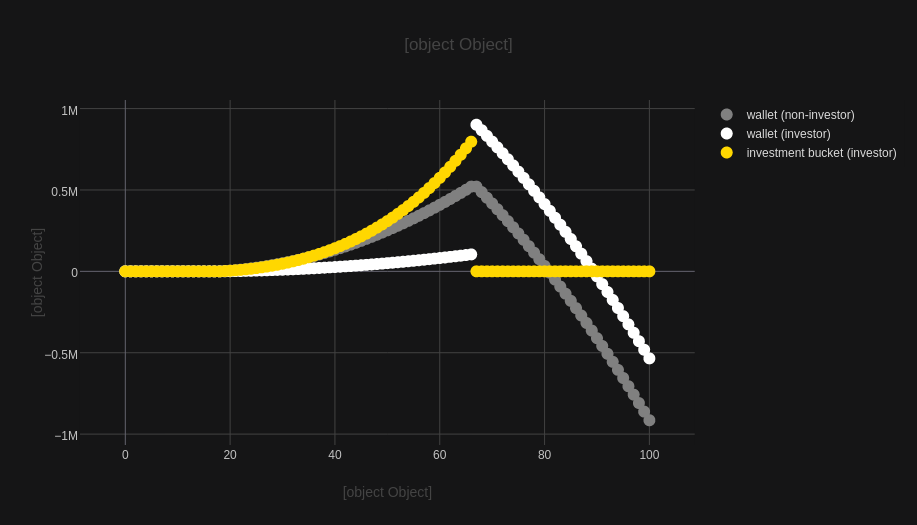
To make it more intuitive, let’s define two $x$ ’s now. Let $x_1$ be the original wallet, while $x_2$ be the investment bucket. In other words, you can think of $x_1$ as your primary bank account, where you receive your salary, pay bills, and taxes, but now you also have the choice to take a certain fraction $\beta \in [0, 1]$ to what is left and move it to $x_2$ . Then, with the $x_2$ money, you buy stock, bonds, commodities, real estate, etc. Whatever you do, you continuously (re-)invest $x_2$ assuming some expecting interest rate $R$ and multiply your money.

In this case, initial equation becomes a system of two coupled oridinary differential equations:

$\left\{\begin{matrix} \frac{d}{dt}x_1 &= \Delta(1 - \beta) \\ \frac{d}{dt}x_2 &= \Delta\beta + x_2\ln(1 + R) \end{matrix}\right.$

To account for the new situation, let’s update the code:

1
2
3
4
5
6
7
8
9
10
11
12
13
14
15
16
17
18
19
class Life:
    def __init__(self):
        ...  # as before
        self.investment_fraction = 0.75  # beta
        self.interest_rate = 5  # 5%

    ...  # as before


def live_with_investing(x, t, you):
    balance = you.earn(t) - you.spend(t) - you.pay_taxes(t)
    if t < self.retirement_age:
        x1 = balance * (1 - you.investment_fraction)
        x2 = np.log(1 + 0.01 * you.interest_rate) * x[1] \
           + balance * you.investment_fraction
    else:
        x1 = balance
        x2 = 0
    return [x1, x2]

There is one thing that distinguishes the implementation from the system of equations we just discussed. Here, for the sake of clarity, we assume that your decision of becoming retired is equivalent to withdrawing all of your money from $x_2$ and supplying it back to $x_1$ . In other words, in our simulation, we want to check how much longer you can support yourself with all the accumulated and generated capital.

Consequently, the simulate function also gets updated:

1
2
3
4
5
6
7
8
9
10
11
12
13
14
15
16
17
def simulate(you):
    ...  # t0, t1, t2 - as before

    # non-investor
    x1_0 = np.zeros((t0.shape[0], 1))
    x1_1 = odeint(live_without_investing, 0, t1, args=(you,))
    x1_2 = odeint(live_without_investing, x1_1[-1], t2, args=(you,))

    # investor
    x2_0 = np.zeros((t0.shape[0], 2))
    x2_1 = odeint(live_with_investing, [0, 0], t1, args=(you,))
    x2_2 = odeint(live_with_investing, [x2_1[-1].sum(), 0], t2, args=(you,))

    df0 = pd.DataFrame({'time': t0, 'wallet (non-investor)': x1_0[:, 0], 'wallet (investor)': x2_0[:, 0], 'investment bucket (investor)': x2_0[:, 1]})
    df1 = pd.DataFrame({'time': t1, 'wallet (non-investor)': x1_1[:, 0], 'wallet (investor)': x2_1[:, 0], 'investment bucket (investor)': x2_1[:, 1]})
    df2 = pd.DataFrame({'time': t2, 'wallet (non-investor)': x1_2[:, 0], 'wallet (investor)': x2_2[:, 0], 'investment bucket (investor)': x2_2[:, 1]})
    return pd.concat([df0, df1, df2])

Observe line 12. This is the place, where we set the new initial condition for the third integral $x_1(t_2) + x_2(t_2) \to x_1(t_2)$ .

/assets/financial-independence-ode-python/case-1-investor.png — Figure 3. Example with `investment_fraction = 0.8` and `interest_rate = 3.3%`. Observe that even with so low-interest rate, you buy yourself almost a decade, or conversely, your early retirement becomes much more attainable.

Inflation - your enemy

We have just seen how powerful exponential growth can be. Unfortunately, regardless if you choose to invest or not, there is one factor that is almost surely present, which also possesses the exponential nature but works against you. It’s inflation.

In simple terms, inflation is not the overall increase in prices, but rather money that loses its value with time. An inflation rate of, say 50%, will result in the same banknote having only 2/3 of its earlier purchasing power. Consequently, to account for inflation in our model, instead of keeping the nominal value of the money, but somehow imagining the prices going up, we will rather model is as a negative interest rate – the kind of compound interest that eats away your money.

Using our earlier knowledge, and denoting inflation rate as $\xi$ , we only need to modify the system of equations slightly:

$\left\{\begin{matrix} \frac{d}{dt}x_1 &= (1 - \beta)\Delta - x_1\ln(1 + \xi), \\ \frac{d}{dt}x_2 &= \beta\Delta + x_2\ln(1 + R) - x_2\ln(1 + \xi). \end{matrix}\right.$

Now, pay attention to the terms multiplied by $x_2$ . Using the properties of the logarithm, we can express the two using just one constant,

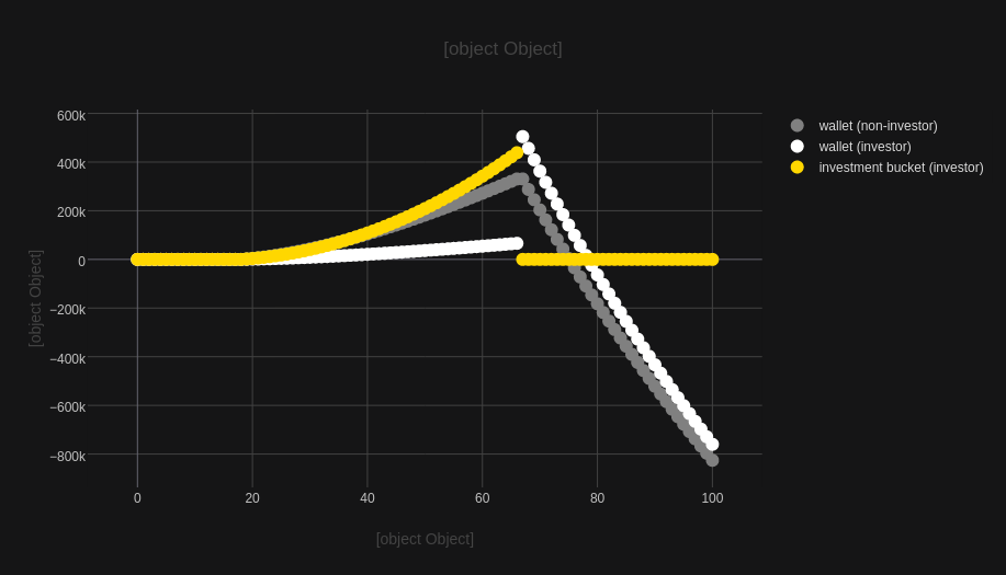
$\ln(1 + R) - \ln(1 + \xi) = \ln\left(\frac{1 + R}{1 + \xi}\right) = \lambda.$

It is now easy to spot, that we can only ever gain on investing if $\lambda > 0$ , which means that we beat the inflation. Naturally, for the “wallet” $x_1$ , our figure is always $\lambda < 0$ , because there is no $R$ to “pull it up”. This is one more reason, why “working hard and saving hard” is a completely hopeless idea.

“Code-wise”:

1
2
3
4
5
6
7
8
9
10
11
12
13
14
15
16
17
18
19
def live_without_investing(x, t, you):
    balance = you.earn(t) - you.spend(t) - you.pay_taxes(t)
    return balance - np.log(1 + 0.01*you.inflation_proc) * x


def live_with_investing(x, t, you):
    balance = you.earn(t) - you.spend(t) - you.pay_taxes(t)
    if t < you.retirement_age:
        x1 = balance * (1 - you.investment_fraction)
        x2 = np.log(1 + 0.01*you.interest_rate_proc) * x[1] \
           + you.investment_fraction * balance
        
        x1 -= np.log(1 + 0.01*you.inflation_proc) * x[0]
        x2 -= x2 - np.log(1 + 0.01*you.inflation_proc) * x[1]
    else:
        x0 = balance
        x1 -= np.log(1 + 0.01*you.inflation_proc) * x[0]
        x2 = 0
    return [x0, x1]

/assets/financial-independence-ode-python/case-2-investor.png — Figure 4. The previous example with `inflation_rate` set to 3.0%, against the `interest rate` set to 3.3%.

Conclusions

In this article, we have shown how you can model your financial situation using ordinary differential equations, as well as how you can turn them into your simulator using python.

The cases discussed here do not consider many factors. The factors such as the tax law in your country, a sudden inheritance, or an inflation spike due to an unexpected financial crisis certainly add to the complexity. What is more, we have not mentioned loans or debts here, although with the approach just presented, we are sure you will be able to include them in your model – and that was precisely the goal of this article.

Finally, as the key take away, especially to those less interested in coding, remember that functions whose growth is proportional to their value are exactly the machinery you want to employ and turn in your favor.

You can also find the notebook that you can run in Google Colab, here: . Feel free to clone it, modify it and play around. Let me know what you think!

Update

Take a look at the newer article, where we try estimate your chances despite life’s unpredictability!