From Matlab towards Python
Intoduction
Life is exciting as it is full of challenges. In my opinion research and development reflects that truth rather well. Few years ago, I faced one when leaving the nice cosy academic environment and begun to work for industry. One of the aspects of that transition was that I could no longer rely on an academic license of Matlab. I took it as a great chance to look for alternatives.
This post, however, is not about Octave, but Python. While Octave is a nice-to-have free alternative to Matlab, I found out it is much more rewarding to invest my time in learning Python on the long run. Indeed, Python is not only free, but also a more standardized, multi-purpose and well-supported language, which may be used for just anything. Having a great community of users, the investment pays real dividends in terms of answers available on fora such as famous StackOverflow.
Please, don’t get me wrong… I still think that Matlab is a great piece of work and I am not advertising for Python at the expense of Matlab, as it is a fine academic tool! However, if you read this, chances are that you might be moving to Python for some reasons, and if your background was Matlab, perhaps you are trying to figure out how you could recreate similar ways and functionalities that you were used to. I believe you just want to concentrate on the “real stuff”, which is your research. If that’s the case, I would like to share some tricks with you. If you are not at all familiar with Matlab, but would like found out more on the similarities and differences, you should benefit too.
What do we cover?
Luckily, both languages are interpreted languages, which makes them work in similar way. They both let us evaluate single lines of code in real time. Still, there are more differences than just syntax. In this post, however, we will not discuss syntax issues, but focus more on the typical routines one follows when working on a code in research context:
- Preparation of work spaces.
- Handling variables.
- Inspection of variables.
- Debugging.
- Saving and loading of variables.
- Building documentation.
Preparation of work spaces
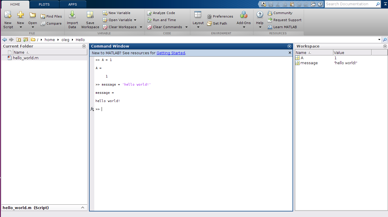
If you were used to starting your day with a cup of tasty coffee and
Matlab environment, we have something in common. Matlab created a very
nice GUI for you to do all the work and focus on what is really important.
Scripts go on the left, variables go on the right, and in between you have
the prompt (>>) and there you go (unless you change it
of course).

In Python, you have a range of options. PyCharm is one of the more popular IDEs with a nice GUI, but personally, I try to avoid using GUI’s for two reasons:
- When moving on to a new problem, I prefer to work with bare-bones software I know (or I am learning). Being forced to learn an IDE takes time, and often it actually obscures my understanding of what is really going on. If every new assignment is a new IDE to learn, it starts to slow me down.
- GUI’s excessively rely on using a mouse. Again, clicking everywhere takes time. Text editors and terminals keep my both hands at the keyboard, often to the point the coffee is getting cold.
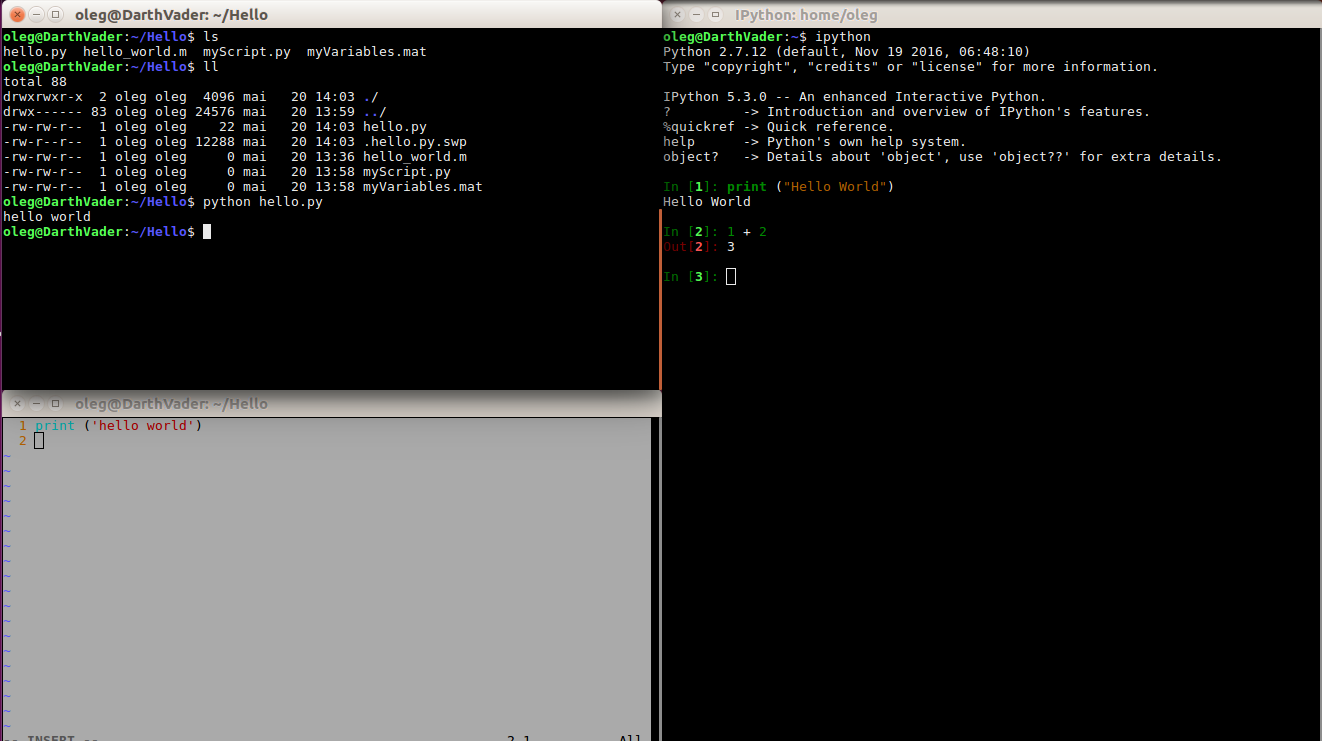
How do we replace this using combination of text editors and terminals? Simply by arranging them in the way we want.

Here, I use a combination of Linux terminals. The one on the right, runs IPython. It is a simple, lightweight Python shell with basic syntax highlighting and auto-completion. It resembles the Matlab shell pretty well. The bottom left part, shows a text editor. Here, I use vim, which is known for its power as well as… rather steep learning curve, but if it is too much, you can use e.g. gedit. Finally, the top left shell I left for just managing the files. If you use Windows, you may use PowerShell and Notepad++. The effect will be very similar.
Now, in contrary to Matlab, IPython would not see the changes to a file if
you edit it using e.g. vim. To enforce the changes, we need to reload
the module, if we run the file through an imported module, or simply
use execfile, which is equivalent to Matlab’s run
command.
Into the code…
You are constructing your library of functions, which you would store
under myLibrary.py. However, you are just experimenting with
the code, checking if it gives you the output you expect. For this reason,
you may create a test script my_test_script.py:
1
2
3
# my_test_script.py
for i in range(a):
    print (i)
Here, we have just a simple loop, but it can be anything. Most importantly, if we save this file (“:w” in vim), all we need to type in IPython is:
a = 10
execfile('my_test_script.py')
Note that having variable a defined in the IPython shell,
we do need to worry that a is unassigned in the test script.
As said before, we may use execfile in Python, just like we
used run in Matlab.
Now, let’s assume that after couple of trials we have an acceptable code
in our test script, we can move it to myLibrary.py and store
it as a function. At this stage, we have got ourselves reusable code
gently stored in one file. In contrary to Matlab, we do not need to
produce copious numbers of files, each containing just one function. All
of the functions can be invoked using import in Python.
...
def print_stupid_loop(limit):
    for i in range(limit):
    print (i)
...
Then in IPython (or some other file):
import myLibrary as mlib
print (mlib.print_stupid_loop(100))
If we wish to change myLibrary.py without restarting
IPython, it is enough we execute:
reload(mlib)to update the work space. As simple as that. Doing this, our workflow is 99% similar to our workflow in Matlab.
Handling of variables - datatypes
There are mainly three types of variables in Matlab. Depending on what you use it for, you may want to store your variable as a:
- matrix - used mainly for numbers, even if it’s just a vector or a scalar,
- cell - for storing all kinds of things, but especially useful for handling strings,
- structure - nice for grouping variables in hierarchical way.
Of course there are also classes, but they often come at a later stage, once the R&D code is more settled and concurrent, and it becomes clearer what part of it will become reused. Until then, it is all building, experimenting, tearing apart and building again. I guess, you’ve been there.
In simple Python, there are three types of array-like things:</p>
- lists - for storing sequences of data (not only numbers) and they are called by their indices,
- dictionaries - similar to lists, but called by keys,
- tuples - similar to the other two, but used as read-only collection of variables.
Although any of them can be applied some basic arithmetic on, they don’t
quite resemble Matlab matrices. Not, until we import numpy. numpy
and scipy are two fundamental modules used in research
within Python. numpy provides basic numerical operations and
scipy can be seen as a more scientific extension providing
support for e.g complex numbers, calculus, etc. Python lists, can easily
be transformed to numpy arrays:
import numpy as np

a = np.array([1, 2, 3])
a_transposed = a.T
...
The syntax is a bit different, but the functionality is essentially the same. For more comparison between the two, you can look here.
Cells and structures can be replaced with dictionaries. A nice advantage of Python is that any strings can be used keys, although I would not recommend using digits only, as that may cause issues when exporting Python variables into Matlab.
Inspection of variables - analytics
You would probably agree that printing data in the interpreter window may
quickly slip control, when data objects begin to contain more and more
numbers. In Matlab, you often create quick plots to peek if a newly
created line of code still makes sense. Here, probably the quickest way is
to invoke pylab which is IPython’s directive that imports numpy
and matplotlib (a module, whose name really speaks for
itself) at once. Having it done, we can easily plot variables in a pretty
Matlab way.
%pylib

a = np.array([1, 2, 3])
b = np.array([1, 4, 7])
plt.plot(a, b)
The matplotlib
module contains numerous functions, and plot is just a simple example. If
more sophisticated analysis is needed, especially handy with “big data”,
it is worth looking at what pandas is to offer. It is Python’s way to do
the analytics.
Debugging
Just before we start, if you heavily rely on visual cues - this red dot in your script, then you’d better use PyCharm. If, on the other hand, you would like to escape the “oppression” of having to work within an IDE, you should consider Python Programming Debugger. It is a native thing, and it will work everywhere. Consider this:
import pdb
import numpy as np
A = np.array([1, 2, 3])
try:
    for i in range(6):
    print (A[i])
except:
    pdb.set_trace()
You know that the loop is bound to fail (IndexError). By combining the try/except
statement and setting the pdb.set_trace() function we set a
break point, which will immediately bring us into the interactive debug
mode and let us use the interpreter to investigate what went wrong. Things
like stepping through the code, continuation, etc. are all there. For a
full list of commands, type ? when in the mode.
In fact, when executing Matlab or Octave with no GUI (through: $./matlab
-nodisplay or $octave --no-gui) this would be the
only way to debug. Essentially, the keyword except would
replaced with catch, the pdb.set_trace() would
be replaced with keyboard and the commands would be prefixed
with db (like dbstep).
Saving and loading
The module we mentioned earlier - scipy - has a function
for storing data as .mat files, which can transport data between the two
worlds. A simple data storage can executed by calling scipy.io.savemat
function:
from scipy.io import savemat
import numpy as np

X = np.array([1, 2, 3])
Y = np.array([3, 2, 1])
Data = {'x':X, 'y':Y}

savemat('test.mat', Data)
This code creates a file Matlab can read. By creating this dictionary, we
will get two matrices x and y, when loading it
into Matlab.
Going backwards is simple too:
from scipy.io import loadmat
import numpy as np

Data = loadmat('test.mat')
print (Data['x'])
print (Data['x'][0])
There is one twist, though. Due to the fact that the basic data storage
unit in Matlab is a matrix (not even a number), calling Data['x']
will return a nested numpy array. In order to
“unfold” it and get it back as we had it, we need to call the first
element of that array to recover our array from within. It is a bit
annoying. I know.
Obviously, when working with more specific things, such as images, sound
samples, databases, and so on, each specific field possesses more natural
ways of storing the data. It is definitely worth looking up scipy
for better ideas.
Documenting
Documenting stuff is always good practice, but it is especially important when working on an R&D related task. Even when it only person reading it may be you at a later stage, pulling together some images, text and snippets of your code can save you hours of frustration when revisiting the same problem twice.
In Matlab, there is an elegant way of transforming your code into
listings, plots into images and comments to text. It is the publish
function that does all the magic of turning your scripts into .html, .pdf,
or .docx outputs. If you haven’t used it, explore it!
Is there a similar way in Python? Of course! Possibly several.
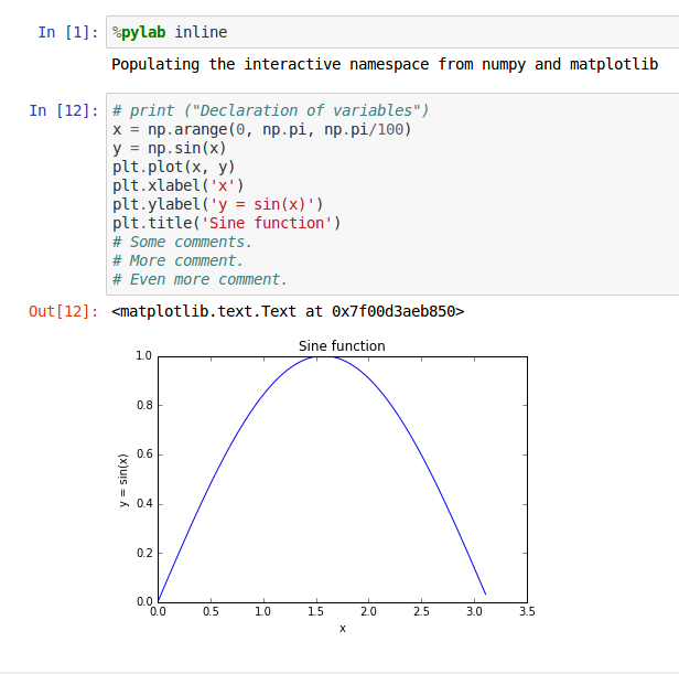
One of the solutions is to take advantage of the web interface to IPython
called Jupyter. It works similar to Wolfram Mathematica,
by letting you segment the execution of the code. For Jupyter to start,
open a terminal and type $ ipython notebook. It will then
open a browser, from which you interactively run pieces of your code. In
order to turn it into documentation, it is enough that instead of typing %pylab,
you type %pylab inline, this will make all of your images
appear in the thread.

Here is just a basic graphical output (e.g. .html) from a Jupyter workspace. Of course, there is more to it, but should provide you with a nice starting point and a base of reference.
Closing remarks
In this post, we have seen how can we quickly find similarities to Matlab in Python. Obviously, when migrating form one environment to the other, it does take a bit of time before becoming fluent. However, I believe that with these bunch of simple tricks, this transition can be fairly smooth and the fluency will eventually come with more time.
