Performance of numpy and pandas - comparison

Introdution

There seems to be no data science in Python without numpy and pandas. (This is also one of the reason why Python has become so popular in Data Science). However, dumping the libraries on the data is rarely going to guarantee the peformance. So what’s wrong?

Let’s begin with the underlying problem. When crafting of an algorithm, many of the tasks that involve computation can be reduced into one of the following categories:

• selecting of a subset of data given a condition,
• applying a data-transforming function onto each data/table entry,
• vector-matrix multiplications (aka typical linear algebra).

In this post, we will try to shed more light on these three most common operations and try to understand of what happens. For all the evaluation of performance, we have used:

• Python version 3.6.7,
• Numpy 1.16.4 and Pandas 0.24.2,
• Ubuntu 16.04,
• PC: Intel Core i5-7200U CPU @ 2.50GHz,
• IPython and %timeit command.

Performance tests

Case 1: Selecting of a subset of data

As for the first case, we select a subset of positive values from a uniformly randomly generated data. Furthermore, we organize the data in form of an numpy array and pandas data frame as either 1-dimentional object of the size of or 2-dimentional array with size of , where is the number of elements. For every , we test the following operations:

1
2
3
4
5
6
7
8
9
10
11
12
13
14
15
16
17
if DIM == 1:
    npx = np.random.randn(N)
else:
    N = int(N**0.5)
    npx = np.random.randn(N, N)
dfx = pd.DataFrame(npx)

%timeit [x > 0 for x in npx]                # explicit loop (DIM == 1)
%timeit [x > 0 for x in [y for y in npx]]   # explicit loop (DIM == 2)

%timeit npx > 0                             # numpy
%timeit np.where(npx > 0, True, False)      # np.where
%timeit dfx > 0                             # dataframe
%timeit dfx.applymap(lambda x: x > 0)       # applymap
%timeit dfx.apply(lambda x: x > 0, axis=0)  # apply, axis=0
%timeit dfx.apply(lambda x: x > 0, axis=1)  # apply, axis=1
%timeit dfx.pipe(lambda x: x > 0)           # pipe

✕

Figure 1.

Selecting a data subset. Left: 1-dimensional array. Right: 2-dimensional array.

First of all, numpy is by all means the fastest. The reason for that it is C-compiled and stores numbers of the same type (see here), and in contrast to the explicit loop, it does not operate on pointers to objects. The np.where function is a common way of implementing element-wise condition on an numpy array. It often comes in handy, but it does come with a small performance price that is related to an overhead of a function call.

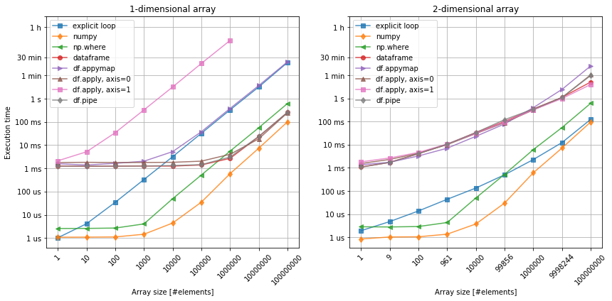
When it comes to the pandas dataframes, their main advantage is the ability to store associated data of different types, which improves both the process of data analysis and code readablility. At the same time, this flexibility is also the main disadvantage of the dataframes when it comes to performance. Looking at the figure 1, we can see that irrespectively of the array size, there is an initial price of 1ms to pay just invoke the calculations. Then, the rest only depends on the array size and… arrangement of its elements!

The x > 0 is a very simple condition that can be applied to any numerical data. Since all our date elements are numbers, it is possible to apply it on all rows (df.apply(..., axis=0), columns (df.apply(..., axis=1)), element-wise (df.applymap) or over the entire dataframe (df.pipe), and so it gives us good way of testing. Comparing 1-dimensional array with 2-dimensional one, we can instanly spot the importance of the axis argument in apply method. Although, our data may not always allow us to choose between these methods, we should try to vectorize along the the shortest axis (columns in this case). If the number of columns and rows are comparable, then df.applymap or df.pipe are better choices.

Last, but not least, it can be noticed that the shape of the array also influences the scaling. Except from numpy (after the initial constant), the execution time on the dataframes is not linear. Still, the possible cross-over between the execution time related to numpy and pandas methods seems to occur in the region of at least elements, which is where cloud computing comes in.

Case 2: Applying atomic function to data

Now, let’s see what it takes to apply a simple atomic calculation: taking a square root of every number. In order to avoid getting into complex numbers, let us use only positive numbers. Furthermore, we introduce vsqrt - a vectorized version of the sqrt function (but not equivalent to np.sqrt) in order to account for the case of bringing a foreign function into numpy. Finally, let’s see the difference between calling sqrt through .apply directly, or through a lambda.

We test the following functions:

1
2
3
4
5
6
7
8
9
10
11
12
13
14
15
16
17
18
19
20
21
if DIM == 1:
    npx = np.random.random((N, 1))
else:
    N = int(N**0.5)
    npx = np.random.random((N, N))
dfx = pd.DataFrame(npx)

def sqrt(x):
    return x**0.5

vsqrt = np.vectorize(sqrt)

%timeit [sqrt(x) for x in npx]                  # explicit loop (DIM == 1)
%timeit [sqrt(x) for x in [y for y in npx]]     # explicit loop (DIM == 2)
%timeit sqrt(npx)                               # numpy
%timeit vsqrt(npx)                              # np.vectorize
%timeit dfx.applymap(sqrt(x))                   # df.applymap
%timeit dfx.apply(sqrt, axis=0)                 # df.apply, axis=0
%timeit dfx.apply(sqrt, axis=1)                 # df.apply, axis=1
%timeit dfx.apply(lambda x: sqrt(x), axis=0)    # df.apply, axis=0, as lambda
%timeit dfx.apply(lambda x: sqrt(x), axis=1)    # df.apply, axis=1, as lambda

✕

Figure 2.

Applying a function to the data. Left: 1-dimensional array. Right: 2-dimensional array.

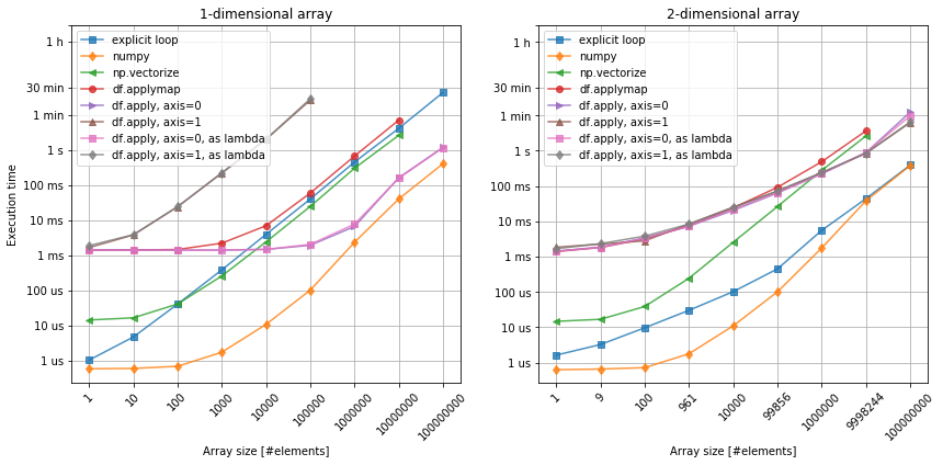
Again, bare-bone numpy beats all the other methods. We can also see the similar behavior of pandas dataframe objects, as comparing with the previous case.

Interestingly, however the vectorized form of the square root function, seems to underperform comparing to the explicit loop. While nearly the same for the 1-dimensional array, for the 2-dimensional case it performs far worse than the loop and even wose than pandas. Perhaps it does make sense, if the original function is relatively more complex, continaing mutliple loops and conditions? Anyway, it seems to be more efficient to just construct function that can be applied directly on the numpy arrays.

Finally, figure 2. shows there is no practical difference between calling df.apply method using lambda or directly. The anonymouns function does offer more flexibiluity (when x becomes row or column), but there is no penalty here.

Case 3: Vector-matrix multiplication

Finally, the last case in this post touches one of the most common numerical operations: calculating a dot-product between a vector and a matrix. Mathematically, this operation can be defined as , where every element of is calculated by taking

,

times, which for array, gives rise to multiplications and additions.

Taking pandas aside for now, numpy already offers a bunch of functions that can do quite the same.

• np.dot - generic dot product of two arrays,
• np.matmul - treating all arrays’ elements as matrices,
• np.inner - alternative to np.dot, but reduced in flexibility,
• np.tensordot - the most generic (generialized to tensors) dot product.

For simplicity, we use a square matrix and compute the product of the following dinemsionality: , yielding operations.

1
2
3
4
5
6
7
8
9
10
11
12
13
14
15
A = np.random.randn(N, N)
X = np.random.randn(N)

def naive(A, X):
    Y = np.zeros(A.shape[1])
    for i in range(A.shape[0]):
        for j in range(A.shape[1]):
            Y[j] += A[i, j]*X[i]
    return Y

%timeit naive(A, X)
%timeit np.dot(A, X)
%timeit np.matmul(A, X)
%timeit np.inner(A, X)
%timeit np.tensordot(A, X, axes=1)

✕

Figure 3.

Vector-matrix multiplication. The black-dotted line denotes the number of operations.

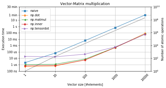
From figure 3, it is evident that custom-made loop-based implementation performs worse by even three orders of magnitude. At the same time, there is no real differnece between the different variants of the dot-product as listed above. The initial flat characteristics can be explained with a penalty associated with a function call itself. The more complicated the function (e.g. np.tensordot), the higher it becomes. However, as soon as the numbers are relatively larger, the execution time is dominated by the actual computation time, which becomes agnosic to the intial funtion.

Conclusions

Having studies the three cases, the following pieces of advice make sense:

• Always use numpy for math and avoid “naive computing”.
• Use preferebly numpy native methods if they exist.
• If they don’t, at least try to encapulate your data in numpy arrays.
• If pandas dataframes are used, make use of apply, applymap and pipe.
• Bear in mind, however, that the shape of a dataframe stongly influences the performance of especially apply method.

So… is your code still running slowly? Look it up again! Maybe it’s not time to move from python to C just yet? Perhaps there is still a method or two that slow the whole thing down, or you have even made a computation hara-kiri?