
Hidden Markov Model - A story of the morning insanity
Introduction
In this article, we present an example of an (im-)practical application of the Hidden Markov Model (HMM). It is an artifially constructed problem, where we create a case for a model, rather than applying a model to a particular case… although, maybe a bit of both.
Here, we will rely on the code we developed earlier , and discussed in the earlier article: “Hidden Markov Model - Implementation from scratch”, including the mathematical notation. Feel free to take a look. The story we are about to tell contains modeling of the problem, uncovering the hidden sequence and training of the model.
Let the story begin…
Picture the following scenario: It’s at 7 a.m. You’re preparing to go to work. In practice, it means that you are running like crazy between different rooms. You spend some random amount of time in each, doing something, hoping to get everything you need to be sorted before you leave.
Sounds familiar?
To make things worse, your girlfriend (or boyfriend) has cats. The little furball wants to eat. Due to the morning hustle, it is uncertain whether you would remember to feed it. If you don’t, the cats will be upset… and so will your girlfriend if she finds out.
Modeling the situation
Say your flat has four rooms. That is to include the kitchen, bathroom, living room and bedroom. You spend some random amount of time in each, and transition between the rooms with a certain probability. At the same time, where ever you go, you are likely to make some distinct kinds of noises. Your girlfriend hears these noises and, despite being still asleep, she can infer in which room you are spending your time.
And so she does that day by day. She wants to make sure that you do feed the cats.
However, since she can’t be there, all she can do is to place the cat food bag in a room where you supposedly stay the longest. Hopefully, that will increase the chances that you do feed the “beast” (and save your evening).
Markovian view
From the Markovian perspective there are rooms are the hidden states ( in our case). Every minute (or any other time constant), we transition from one room to another . The probabilities associated with the transitioning are the elements of matrix .
At the same time, there exist distinct observable noises your girfriend can hear:
- flushing toilet (most likely: bathroom),
- toothbrushing sound (most likely: bathroom),
- coffee machine (most likely: kitchen),
- opening the fridge (most likely: kitchen),
- TV commercials (most likely: living room),
- music on a radio (most likely: kitchen),
- washing dishes (most likely: kitchen),
- taking a shower (most likely bathroom,
- opening/closing a wardrobe (most likely: bedroom),
- ackward silence… (can be anywhere…).
The probabilities of their occurrence given a state is given by coefficients of the matrix . In principle, any of these could originate from you being in an arbitrary room (state). In practice, however, there is physically a little chance you pulled the toilet-trigger while being in the kitchen, thus some ’s will be close to zero.
Most importantly, as you hop from one room to the other, it reasonable to assume that whichever room you go to depends only on the room that you have just been to. In other words, the state at time depends on the state at time only, especially if your are half brain-dead with an attention span of a gold fish…
Uncovering the hidden states
The goal
For the first attempt, let’s assume that the probability coefficients are known. This means that we have a model , and our task is to estimate the latent sequence given the observation sequence, which corresponds to finding . In other words, the girlfriend wants to establish in what room do we spend the most time, given what she hears.
Initialization
Let’s initialize our and .
| bathroom | bedroom | kitchen | living room | |
|---|---|---|---|---|
| bathroom | 0.90 | 0.08 | 0.01 | 0.01 |
| bedroom | 0.01 | 0.90 | 0.05 | 0.04 |
| kitchen | 0.03 | 0.02 | 0.85 | 0.10 |
| living room | 0.05 | 0.02 | 0.23 | 0.70 |
| coffee | dishes | flushing | radio | shower | silence | television | toothbrush | wardrobe | |
|---|---|---|---|---|---|---|---|---|---|
| bathroom | 0.01 | 0.01 | 0.20 | 0.01 | 0.30 | 0.05 | 0.01 | 0.40 | 0.01 |
| bedroom | 0.01 | 0.01 | 0.01 | 0.10 | 0.01 | 0.30 | 0.05 | 0.01 | 0.50 |
| kitchen | 0.30 | 0.20 | 0.01 | 0.10 | 0.01 | 0.30 | 0.05 | 0.02 | 0.01 |
| living room | 0.03 | 0.01 | 0.01 | 0.19 | 0.01 | 0.39 | 0.39 | 0.01 | 0.03 |
| bathroom | bedroom | kitchen | living room |
|---|---|---|---|
| 0 | 1 | 0 | 0 |
1
2
3
... # all initializations as explained in the other article
hml = HiddenMarkovLayer(A, B, pi)
hmm = HiddenMarkovModel(hml)
Simulation
Having defined and , let’s see how a typical “morning insanity” might look like. Here, we assume that the whole “circus” lasts 30 minutes, with one-minute granularity.
1
2
observations, latent_states = hml.run(30)
pd.DataFrame({'noise': observations, 'room': latent_states})
| t | noise | room |
|---|---|---|
| 0 | radio | bedroom |
| 1 | wardrobe | bedroom |
| 2 | silence | bedroom |
| 3 | wardrobe | bedroom |
| 4 | silence | living room |
| 5 | coffee | bedroom |
| 6 | wardrobe | bedroom |
| 7 | wardrobe | bedroom |
| 8 | radio | bedroom |
| 9 | wardrobe | kitchen |
| … | … | … |
The table above shows the first ten minutes of the sequence. We can see that it kind of makes sense, although we have to note that the girlfriend does not know what room we visited. This sequence is hidden from her.
However, as it is presented in the last article, we can guess what would be the statistically most favorable sequence of the rooms given the observations.
The problem is addressed with the .uncover method.
1
2
estimated_states = hml.uncover(observations)
pd.DataFrame({'estimated': estimated_states, 'real': latent_states})
| t | estimated | real |
|---|---|---|
| 0 | bedroom | bedroom |
| 1 | bedroom | bedroom |
| 2 | bedroom | bedroom |
| 3 | bedroom | bedroom |
| 4 | bedroom | living room |
| 5 | bedroom | bedroom |
| 6 | bedroom | bedroom |
| 7 | bedroom | bedroom |
| 8 | bedroom | bedroom |
| 9 | bedroom | kitchen |
| … | … | … |
Comparing the results, we get the following count:
| estimated time proportion | real time proportion | |
|---|---|---|
| bathroom | 1 | 2 |
| bedroom | 18 | 17 |
| kitchen | 4 | 10 |
| living room | 8 | 2 |
The resulting estimate gives 12 correct matches. Although this may seem like not much (only ~40% accuracy), it is 1.6 times better than a random guess.
Furthermore, we are not interested in matching the elements of the sequences here anyway. What interests us more is to find the room that you spend the most amount of time in. According to the simulation, you spend as much as 17 minutes in the bedroom. This estimate is off by one minute from the real sequence, which translates to ~6% relative error. Not that bad.
According to these results, the cat food station should be placed in the bedroom.
Training the model
In the last section, we have, relied on an assumption that the intrinsic probabilities of transition and observation are known. In other words, your girlfriend must have been watching your pretty closely, essentially collecting data about you. Otherwise, how else would she be able for formulate a model?
Although this may sound like total insanity, the good news is that our model is also trainable. Given a sequence of observations, it is possible to train the model and then use it to examine the hidden variables.
Let’s take an example sequence of what your girlfriend could have heard some crazy Monday morning. You woke up. Being completely silent for about 3 minutes, you went about to look for your socks in a wardrobe. Having found what you needed (or not), you went silent again for five minutes and flushed the toilet. Immediately after, you proceeded to take a shower (5 minutes), followed by brushing your teeth (3 minutes), although you turn the radio on in between. Once you were done, you turned the coffee machine on, watched TV (3 minutes), and did the dishes.
So, the observable sequence goes as follows:
1
2
3
4
5
6
7
8
9
10
11
12
13
what_she_heard = ['silence']*3 \
+ ['wardrobe'] \
+ ['silence']*5 \
+ ['flushing'] \
+ ['shower']*5 \
+ ['radio']*2 \
+ ['toothbrush']*3 \
+ ['coffee'] \
+ ['television']*3 \
+ ['dishes']

rooms = ['bathroom', 'bedroom', 'kitchen', 'living room']
pi = PV({'bathroom': 0, 'bedroom': 1, 'kitchen': 0, 'living room': 0})
The starting point is the bedroom, but and are unknown. Let’s initialize the model, and train it on the observation sequence.
1
2
3
4
5
6
7
8
9
10
11
12
13
14
np.random.seed(3)
model = HiddenMarkovModel.initialize(rooms,
list(set(what_she_heard)))
model.layer.pi = pi
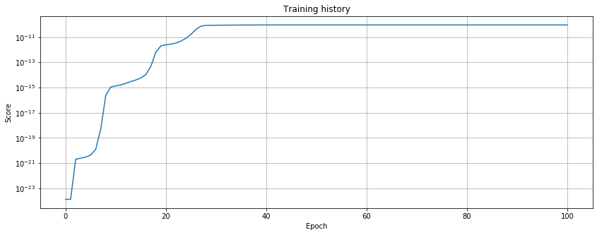
model.train(what_she_heard, epochs=100)
fig, ax = plt.subplots(1, 1, figsize=(10, 5))
ax.semilogy(model.score_history)
ax.set_xlabel('Epoch')
ax.set_ylabel('Score')
ax.set_title('Training history')
plt.grid()
plt.show()
Now, after training of the model, the prediction sequence goes as follows:
1
2
3
4
pd.DataFrame(zip(
	what_she_heard,
	model.layer.uncover(what_she_heard)),
	columns=['the sounds you make', 'her guess on where you are'])
| t | the sound you make | her guess on where you are |
|---|---|---|
| 0 | silence | bedroom |
| 1 | silence | bedroom |
| 2 | silence | bedroom |
| 3 | wardrobe | bedroom |
| 4 | silence | bedroom |
| 5 | silence | bedroom |
| 6 | silence | bedroom |
| 7 | silence | bedroom |
| 8 | silence | bedroom |
| 9 | flushing | bathroom |
| 10 | shower | bathroom |
| 11 | shower | bathroom |
| 12 | shower | bathroom |
| 13 | shower | bathroom |
| 14 | shower | bathroom |
| 15 | radio | kitchen |
| 16 | radio | kitchen |
| 17 | toothbrush | living room |
| 18 | toothbrush | living room |
| 19 | toothbrush | living room |
| 20 | coffee | living room |
| 21 | television | living room |
| 22 | television | living room |
| 23 | television | living room |
| 24 | dishes | living room |
| state (guessed) | total time steps |
|---|---|
| bathroom | 6 |
| bedroom | 9 |
| kitchen | 2 |
| living room | 8 |
According to the table above, it is evident that the cat food should be placed in the bedroom.
However, it is important to note that this result is somewhat a nice coincidence because the model was initialized from a purely random state. Consequently, we had no control over the direction it would evolve in the context of the labels. In other words, the naming for the hidden states is are simply abstract to the model. They are our convention, not the model’s. Consequently, the model could have just as well associated “shower” with the “kitchen” and “coffee” with “bathroom”, in which case the model would still be correct, but to interpret the results we would need to swap the labels.
Still, in our case, the model seems to have trained to output something fairly reasonable and without the need to swap the names.
Conclusion
Hopefully, we have shed a bit of light into this whole story of morning insanity using the Hidden Markov model approach.
In this short story, we have covered two study cases. The first case assumed that the probability coefficients were known. Using these coefficients, we could define the model and uncover the latent state sequence given the observation sequence. The second case represented the opposite situation. The probabilities were not known and so the model had to be trained first in order to output the hidden sequence.
Closing remark
The situation described here is a real situation that the author faces every day. And yes… the cats survived. ;)